Basics of NLP - 3 [Week 7]
a guide into how hidden markov models, text clustering, attention work
This is the last part of the NLP series. Please read the earlier two first
Check that out : Basics of NLP - 1 [Week 5], Basics of NLP - 2 [Week 6]
Let’s continue from where we left off.
This blog is broken into 3 pieces
- Hidden Markov Models
- Text Clustering
- Attention Mechanism
Hidden Markov Models
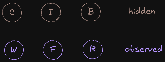
In such models, we work with two kinds of variables — hidden and observed.
Like the name suggests, the hidden states are never observed by us, but we get information about them by observing the observed variables, which are emitted by the hidden state. Confusing right?
Let’s use an example
The Intuition
Meet my friend Aakash 👨🔬. He is a peculiar one. His appetite depends on how the weather is. He decides what he wants to eat, based on what the weather is.
As you can notice, I can’t observe what he wants to eat, but I can clearly observe what the weather is outside. So,
Hidden Variable - What Aakash is going to eat
Observed Variable - What the weather is
Let’s define the variables
| Hidden | Observed |
|---|---|
| Chai (C) | Warm (W) |
| Ice Cream (I) | Frigid (F) |
| Biriyani (B) | Rainy (R) |
The Probability Tables
The next step is to create two tables - Transition Table and Emission Table
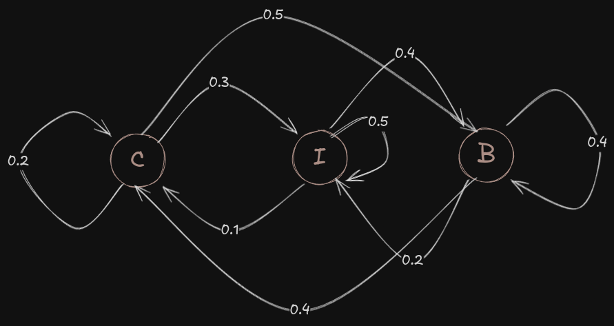
State Transition Table
This table decides the transitions between all the hidden states. Theoretically, you can have a transition from any state to any other state. Let’s make one for our use case.
| Start/End | C | I | B |
|---|---|---|---|
| C | 0.2 | 0.3 | 0.5 |
| I | 0.1 | 0.5 | 0.4 |
| B | 0.4 | 0.2 | 0.4 |
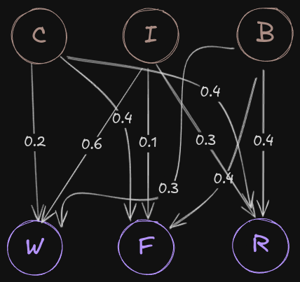
State Emission Table
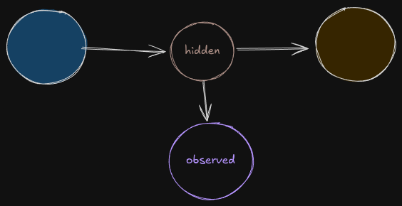
Now of course, hidden states will be related to the observation table in some way, every transition to hidden state emits observation symbol.
| Start/End | W | F | R |
|---|---|---|---|
| C | 0.2 | 0.4 | 0.4 |
| I | 0.6 | 0.1 | 0.3 |
| B | 0.3 | 0.4 | 0.4 |
Additional Stuff
We are gonna study about two things - initial state and terminal state. They both are mainly used for internal calculations and help us while building HMMs
Initial State and Terminal State
Let’s say you emit a signal named R, for it to happen there has to be some transition to the hidden state. So where does it start from? That’s where initial state comes into play! In the earlier state emission diagram, you can see the probability of which hidden state will emit R, but from what state that transition happened, we don’t know, we name it as initial state.
When you reach the end of the observation sequence you basically transition to the terminal state, because every observation sequence is processed as separate units. The probability of this will always be one (why? This is an exercise)

Observation Sequence
This is a sequence of observation symbols from 1 symbol to N symbols. When we write a sequence, the units don’t know about the past or the future, this is because we need to know the initial and terminal states for that.
Text Clustering
Clusters are basically groups of same type of objects. Now when we do clustering, what we mean is to separate items into these groups. We try to put new, unseen objects into their respective groups. Here, there will be no exact number of clusters, you can decide any number according to your preference!
Clusters can either be hard or soft. In hard clustering, every object belongs to one and only one cluster, while in soft clustering, it can belong to as many clusters as it wants to(as in, there exists some intersection between the clusters)
How do we cluster?
It has few steps to itself,
- Feature Selection - We try to select only the most important features and try to with those data features only.
- Clustering Algorithm - We decide to use any algorithm to do the clustering (we will go in detail about this)
- Data Abstraction - We try to find out the meaning behind each cluster, as in what Cluster A indicates.
- Final Step - Finally, we derive our required results from this process
Word Clustering
This is nothing but a discussion of text preprocessing and Word2Vec [Please read it from Blog 1]
Clustering Documents
This is nothing but a discussion of tf-idf [Please read it from Blog 1]
K Means
It is one of the most famous clustering algorithms.
It assigns k random points in the space, initially. Then it assigns each data point to it’s nearest mean of clusters. The actual mean is then calculated, based on how much the means are shifted, the data points get arranged differently. The process is repeated till the means stop moving.
For a more detailed explanation, see this video by CampusX K-Means Clustering Algorithm | Geometric Intuition | Clustering | Unsupervised Learning
Latent Dirichlet Allocation (LDA)
On many occasions, just clusters existing isn’t enough for us.
We assume two things -
- Each document has a distribution over some topics
- Each topic will have a distribution over the words
What is it?
Latent means hidden variables, Dirichlet hints towards the probability distribution over some other probability distribution, and Allocation indicates we are allocating some values concerning the earlier ones.
To explain this in detail, the blog will get very long.
I am linking a very intuitive blog in that respect here :)
Link - Latent Dirichlet Allocation(LDA)
Attention Mechanism
Before going in-depth, let’s visit Seq2Seq and RNNs.
Seq2Seq And RNNs
Paper Link - Sequence to Sequence Learning with Neural Networks
My Blog on RNNs - RNNs [Week 4]
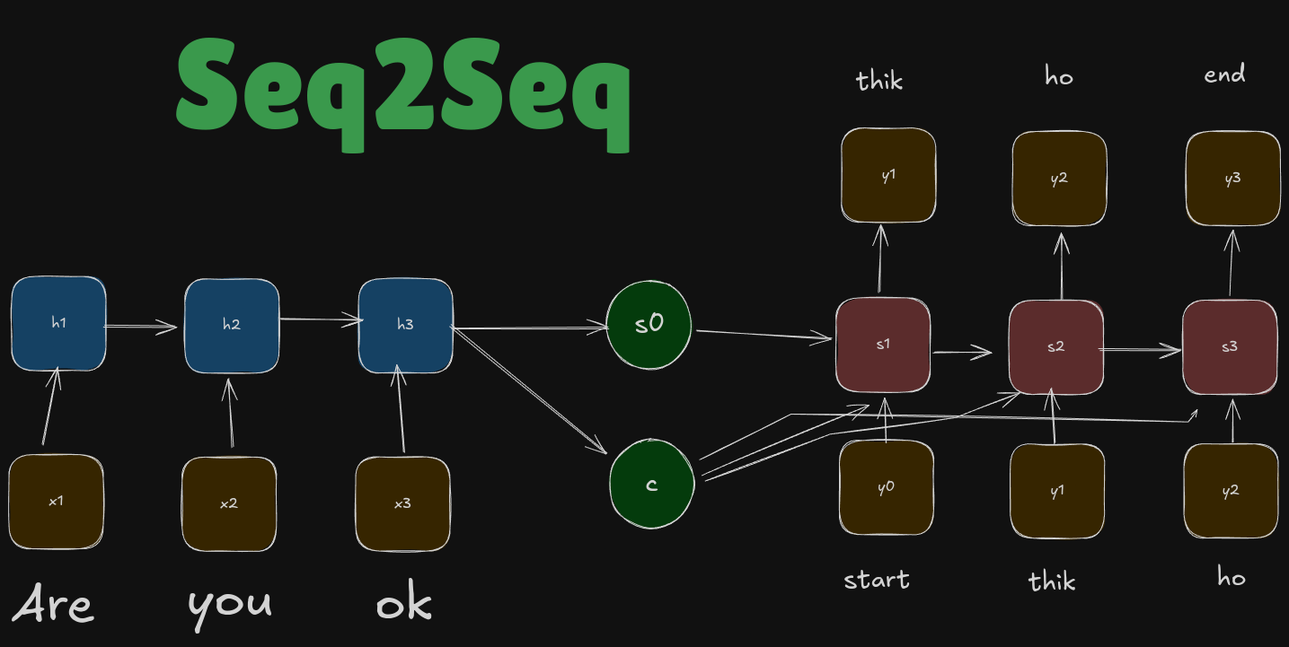
We have two sections - Encoder RNN and Decoder RNN.
The encoder processes the input and generates a context vector c, which includes all the essential information from the input and also generates an initial decoder state, \(s_0\). The decoder uses this context vector to produce the output sequence step by step, relying on it’s previous outputs and content vector at each step. [We will not go into too much detail as it will take up a lot of blog time]
This kind of solution is good, if we are working with smaller samples, but if we have bigger samples, then the context vector is not able to hold all meaningful information from our encoder part. This is called the bottleneck problem, which is basically the loss of information in the fixed-size context vector! For example
The sun dipped below the horizon, painting the sky in hues of orange and purple. A gentle breeze rustled the leaves, whispering secrets of the day. Children laughed as they played, their joy infectious. In this serene moment, nature and humanity intertwined, reminding us of life’s simple yet profound beauty. ~ ChatGPT 2024
To make a context vector of this quote, we’d need a very long context vector, hence we need to fix this issue.
With Attention what we aim to do is, try to create a new context vector at every timestep of the decoder which will give meaning different to each encoded sequence.
What is Attention
Paper Link - Neural Machine Translation by Jointly Learning to Align and Translate
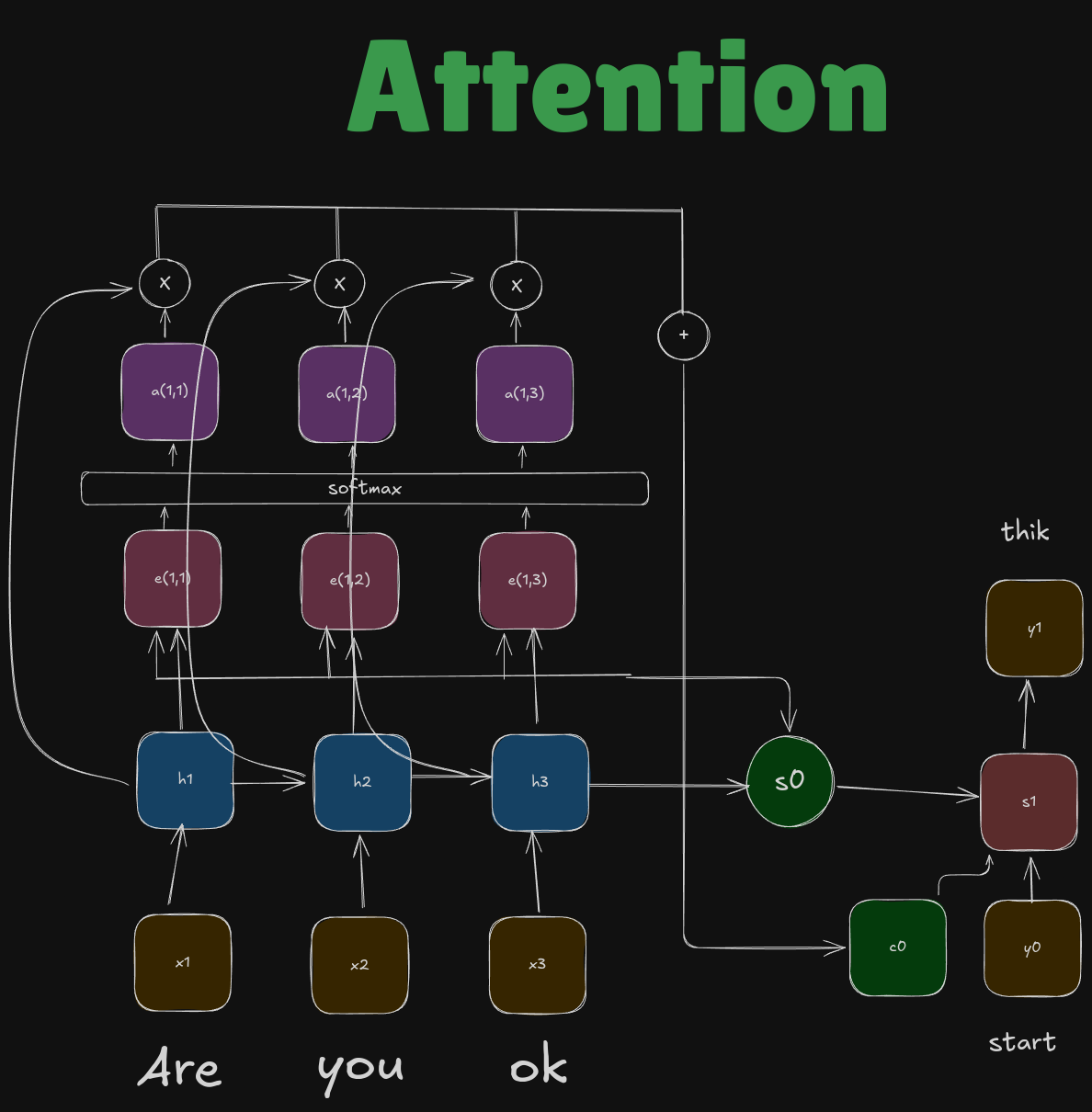
Let’s dissect this at \(t=1\)
E Score
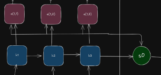
At \(T=t\), we use \(s_{t-1}\) decoder state to find \(e\) . We use a special function \(f\) to compute the value of e.
This function is nothing but a multilayer perception function. It is also called the alignment function.
The numbers are some scalar values that tell us how \(h_1\) is contributing to predict \(s_0\). Since they are scalar values, we must normalize them by applying softmax function.
Attention Score
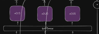
The final result we get after applying the softmax function for each value is called the attention score. They tell us how the hidden state is related to the final \(s_0\) decoder state.
Final Context Vector
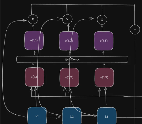
This works in 3 steps.
Step 1
Take the hidden vectors and multiply them with their respective attention weights.
Step 2
Compute the result for each of the attention weights and hidden weights.
Step 3
Add all the results up to get your context vector.
Repeat This
What I did was do the first step. What you’ve to do is to do it for every step, two more times.
Find the \(e, a,c\) for \(t=2,3\) and then consecutively find \(y_2,y_3,y_4\). The method is the same as I have discussed earlier
Exercise: Actually code the whole attention thing using just numpy
Attention Layer
Now that we know what attention is, let’s try to make an attention layer.