RNNs [Week 4]

a deep dive into recurrent neural networks and how the math behind it works

Intuition

Let’s say you are thinking of something.

I want to have some ice cream as it is very hot.

Notice how you thought of ice creams when you noticed that it is very hot outside. We, as humans, form thoughts, based on a pre processed thought. You will never have a blank mind and think stuff from literally nothing. In simple words, your words have some persistence.

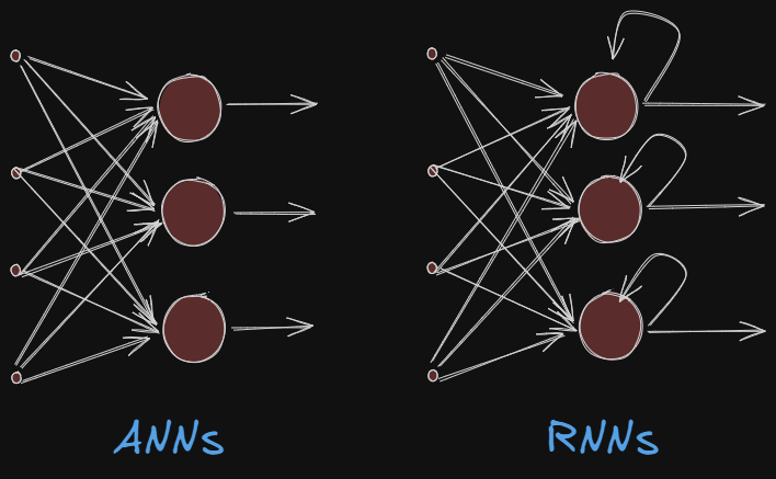
Artificial Neural Networks fail to capture this beautiful thing. It fails to use its reasoning about previous events to learn facts that will inform the later events. We lose the context or sequential information. Additionally ANNs have lots of unnecessary padding which will need extra compute.

This is where Recurrent Neural Networks(RNN) come in.

Unlike traditional neural networks where each input is independent, RNNs can access and process information from previous inputs. This allows it to handle sequential data.

Extra : Sequential Data

This kind of data is a type of information in which order matters. Each data is connected to the earlier data. Without this connection there is no context and the data becomes meaningless.

I to have ice as is cream very hot it some want.

Makes no sense right? The order of the words give context to the sentence. This kind of sequential data is called Natural Language Text. If we use this sentence as some kind of speech and speak it out with correct syllables and pronunciation, it becomes a Speech Signal.

Any kind of signal that varies as \(f(t)\) can be coined as a type of sequential data, popularly called as Time Series.

Types of RNNs

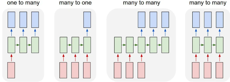
One to Many

A one-to-many architecture represents a scenario where the network receives a single input but generates a sequence of outputs.

The RNN takes in a single piece of info as input, maybe something like image. Then the RNN processes the input and generates a sequence of outputs over time!

Applications

Music Generation : RNN Input is one single music note, from which it generates a sequence of notes forming a musical masterpiece
Image Captioning : RNN Input is one single image, from which it generates a paragraph of text describing the image.

Many to One

A many-to-one architecture represents a scenario where the network receives a sequence of inputs but generates a single outputs.

The RNN takes in a sequence of data points over time, which could be data points for a stock over few hours. Then it generates a single output value, which could be a classification, or a prediction, or even a summary.

Applications

Spam Detection : RNN Input is a sequence of words in the email content, from which it classifies it to tell if it’s spam or not(single output).
Financial Predictions : RNN Input is a sequence of data points from a stock price, from which it predicts what the next stock price might be(single output).

Many to Many

A many-to-many architecture represents a scenario where the network receives a sequence of inputs and generates a sequence of outputs.

The RNN takes in a sequence of data points over time, which could be words in a sentence for example. Then, the RNN generates a new sequence of data points, with a length that may or may not be the same as the input sequence.

Types

Variable Length : The output sequence has a different length as compared to the input. Usually used in machine translation.
Fixed Length : The output sequence has the same length as the input sequence. A very common example is named entity recognition(NER).

Applications

Video Captioning : RNN input is a sequence of images, from which it gives a paragraph describing it.
Machine Translation : RNN input is a sequence of words in Language A, from which it gives an output of another sequence of words in Language B.

Working Principle

Parts

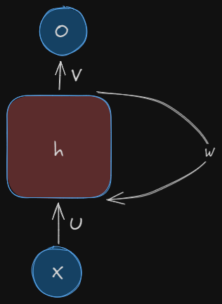
This is how an RNN looks like. Looks confusing right? Let’s unfold this.

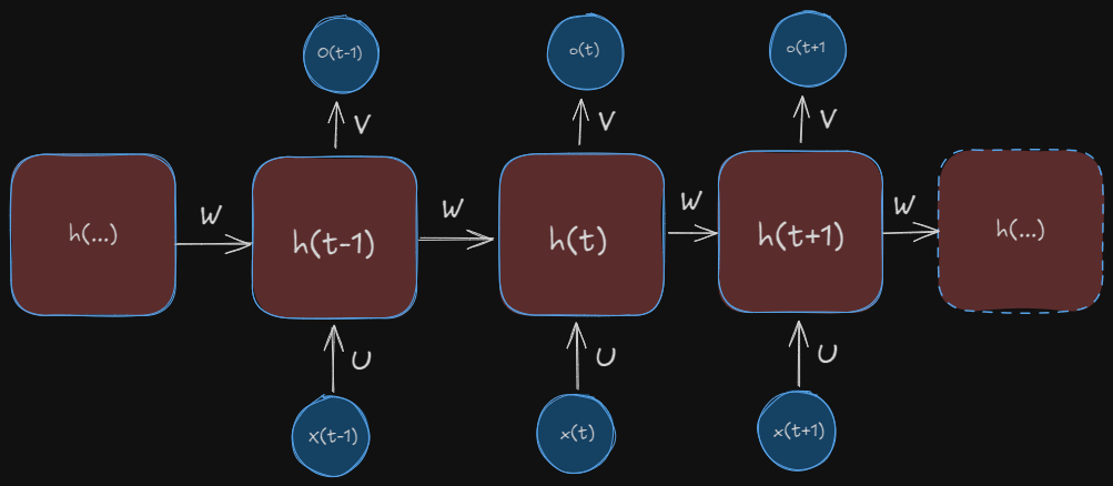
This is an RNN in it’s unfolded state, where we write out the network’s complete sequence. For example, if our RNN has 4 data points, our unfolded version should be 4 layers deep.

\(x(t)\) is the input taken by the RNN at time \(t\). We usually take one-hot vectors in case of words in a sentence as input for the RNNs.

\(h(t)\) is called the hidden state of the RNN at time \(t\). It is kind of like the memory of the RNN. It’s calculation is done by the inputs of the current input and the hidden state of the earlier block. We will discuss them in detail later

\[h(t+1)=f(\alpha x(t)+\beta h(t-1))\]

The RNN has input to hidden connections parameterized by a \(U\), hidden-to-hidden recurrent connections parameterized by \(W\), and hidden-to-output connections parameterized by a \(V\)and all these weights \((U,V,W)\) are shared across time.

\(o(t)\) is the output the RNN at time \(t\).

Forward Propagation

Let’s dissect how a RNN looks from within first.

Some Assumptions

The output is discrete, as we are trying to predict words or something.
Use \(tanh\) function for activation layer

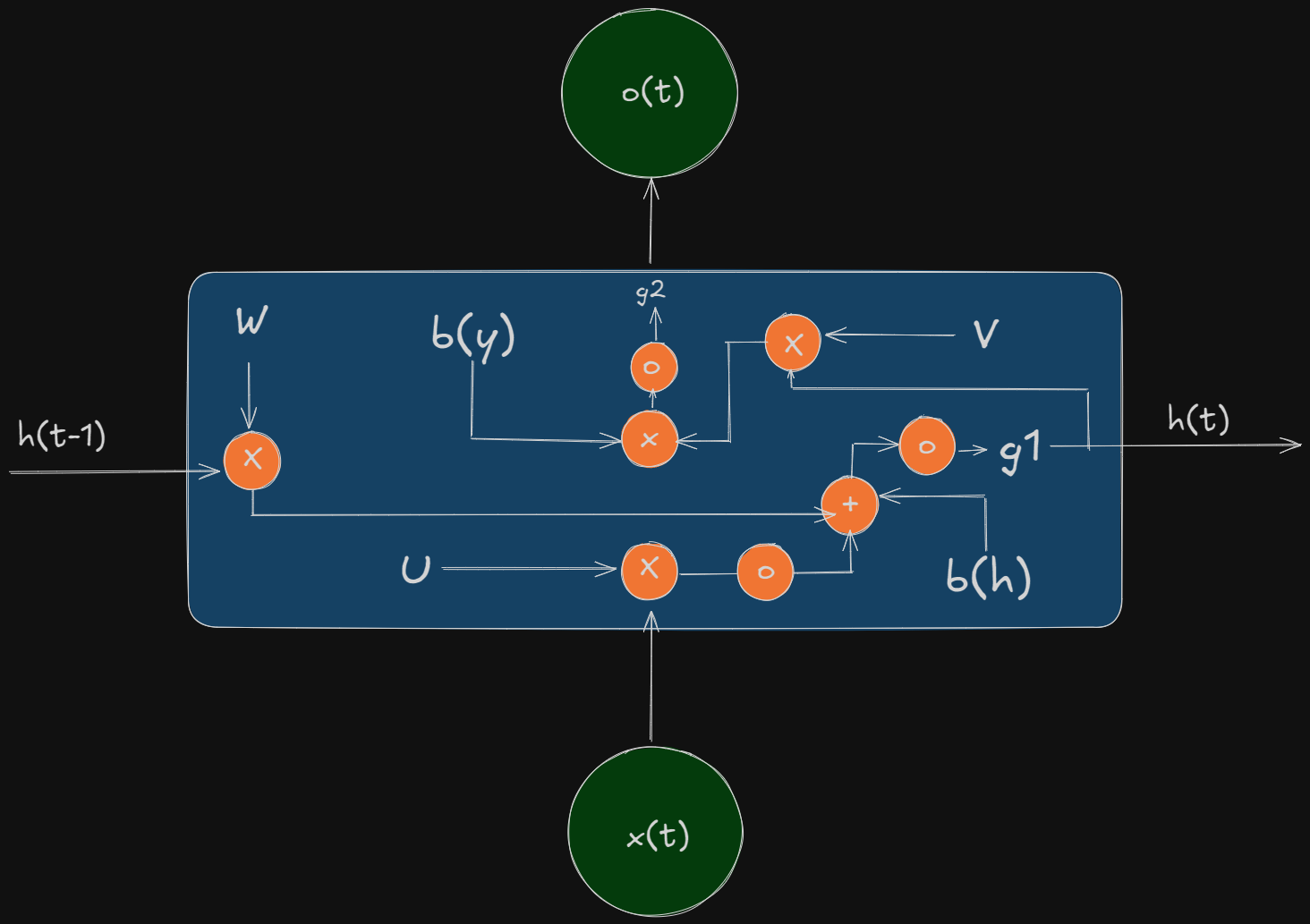
The Math

First we take the values \(h_{t-1}\) and \(W\) and multiply them. We also multiply \(U\) and \(x_t\), then we consider a bias term of \(b_h\)(apply the first activation here).

We add them up and we will be using the the activation function of \(tanh\) for \(g_1\)

\[h_t=tanh(W .\space h_{t-1}+U.\space x_t+b_h)\]

To find the output \(o_t\), we multiply our result \(h_t\) with V and then add it with the bias term. The last activation function is nothing but a \(softmax\).

\[o_t=softmax(V.\space h_t+b_y)\]

Backward Propagation

The back-propagation algorithm applied to the unfolded graph here is called backpropagation through time. As the parameters are shared by the all time steps, the gradient of the output depends not only on the current time step, but also on the previous time steps.

Let’s refine some stuff so it’s easier for us to understand what each math term means(trust me there’s a lot)

Math Term	Meaning
x(t)	input at t
a0	first activation
h(t)	rnn output at t
W(x), b(x)	weights and biases at input
W(y), b(y)	weights and biases at output
W(h), b(h)	weights and biases at rnn
y’(t)	prediction at time t
L	loss function
σ(i)	activation of ith layer
σ’(i)	derivation of activation of ith layer
U(h)	recurrent weights
δ(Loss)	derivative of loss(arbitary)

Now we know from the previous forward pass :

\[a^0_t=\sigma_0(x_tW_x^T+b_x)\\ h_t=\sigma_1(a_t^0W_h^T+h_{t-1}U_h^T+b_h)\\ \hat{y}_t=\sigma_2(h_tW_y^T+b_y)\\ L=f(\hat{y}_t,y_t)\]

Don’t get scared by looking at these equations, what you learnt earlier is exactly the same thing - just variables have changed.
Also we just broke the earlier three activations into three equations, nothing else

Gradient Rule for \(\hat{y}_t\)

We have taken the loss function to be arbitary, it can be anything you want. We will be going forward with L2 loss here. For that reason we’ll just keep the derivative of Loss as \(\delta\).

First let’s find a chain rule w.r.t to \(W_{y_t}\)

\[\frac{\delta \mathcal{L}}{\delta W_{y_t}} = \frac{\delta \mathcal{L}}{\delta \hat{y}_t} \frac{\delta \hat{y}_t}{\delta W_{y_t}} \\= [\delta_t^{Loss} .\space \sigma_2'(h_t W_{y_t}^T + b_{y_t})]^T h_t = [\delta_t^{Loss} .\space \sigma_2'(z_{y_t})]^T h_t\\ \\ \]

How did we get this? Let’s break part by part.
Our Loss function is :

\[\mathcal{L} = \frac{1}{N} \sum_{t=1}^{N} (y_t - \hat{y}_t)^2\]

Our gradient with \(\hat{y}_t\) comes out to be :

\[\frac{\delta \mathcal{L}}{\delta \hat{y}_t} = -\frac{2}{N}(y_t - \hat{y}_t)\]

And the second part of the chain rule is :

\[\frac{\delta \hat{y}_t}{\delta W_{yt}} = h_t^T[\sigma_2'(z_{yt})]\]

→ where \(z_{y_t}\) is just \(h_tW_y^T+b_y\)

Combining these results, and after doing some calculations, we get :

\[\frac{\delta \mathcal{L}}{\delta W_{yt}} = [\delta_t^{Loss} .\space \sigma_2'(z_{y_t})]^T h_t\\ \\\]

Now let’s find a chain rule w.r.t to \(b_{y_t}\)(not explaining this in detail as it’s similar to the earlier one)

\[\frac{\delta \mathcal{L}}{\delta b_{y_t}} = \frac{\delta \mathcal{L}}{\delta \hat{y}_t} \frac{\delta \hat{y}_t}{\delta b_{y_t}}\\ = \sum_{} [\delta_t^{Loss} .\space\sigma_2'(h_t W_{y_t}^T + b_{y_t})] = \sum_{} [\delta_t^{Loss} .\space\sigma_2'(z_{y_t})]\]

Let’s now try to find \(\delta^ \mathcal{L-1}_{t} \), which is basically just passing the gradient of the loss to the earlier RNN Layer.

\[\delta^ \mathcal{L-1}_{t} = \frac{\delta \mathcal{L}}{\delta \hat{y}_t} \frac{\delta \hat{y_t}}{\delta h_t}\]

Now we know :

\[\frac{\delta \hat{y}_t}{\delta h_t} = W_{y_t}^T \sigma_2'(z_{yt})\]

So finally,

\[\delta^ \mathcal{L-1}_{t}= [\delta_t^{Loss} . \space \sigma_2'(z_{yt})]W_{yt}\]

Gradient Rule for the RNN

How is RNN different from normal neural networks, if we are just using normal gradient descent?
The answer is simple, here we send the gradient of the hidden state back through time and its added on with the earlier gradients. Let’s see it mathematically.

We know,

\[h_t=\sigma_1(a_t^0W_h^T+h_{t-1}U_h^T+b_h)\]

Let \(a_t^0W_h^T+h_{t-1}U_h^T+b_h=K\), and then :

\[\frac{\delta h_t}{\delta h_{t-1}} = \frac{\delta}{\delta h_{t-1}}[\sigma_1(K)]\\ \frac{\delta h_t}{\delta h_{t-1}} = \sigma_1'(K) \cdot \frac{\delta K}{\delta h_{t-1}}\]

Now let’s try to find \(\frac{\delta K}{\delta h_{t-1}}\)

\[\frac{\delta K}{\delta h_{t-1}}=\frac{\delta (a_t^0W_h^T+h_{t-1}U_h^T+b_h)}{\delta h_{t-1}}\\ =U_h^T\]

After combining the results, we finally get :

\[\frac{\delta h_t}{\delta h_{t-1}} = \sigma'_1(K)U_h^T\]

This is the value that we send through the BPTT time steps, till we get to the first one. How we store the values, is by adding it to the earlier one. To get the previous step, we just need to add \(\frac{\delta h_{t-1}}{\delta h_{t-2}}\)to our earlier result.

This addition is repeated till \(t=0\), after which this sum variable is made to be 0.