LLMs - 2 [Week 10]

Please read the first part before getting into this blog
LLMs - 1 [Week 8]

All About Attention

We had covered the data preprocessing part earlier on, now we must learn a very essential part of a LLM - Attention. Let’s get a deep dive through history how we came across attention and why did we even need it in the first place!

This blog will be broken into 8 parts :

• Problems with RNNs, and how it led to attention
• Bahadanau Attention
• Attention Layer (Single Head Attention)
• Masked Attention
• Multi Head Attention
• Grouped Query and Multi Query Attention
• Cross Attention
• Soft and Hard Attention

Why did we need Attention

The latest technology before attention was Seq2Seq. We need to figure out how did it fail?

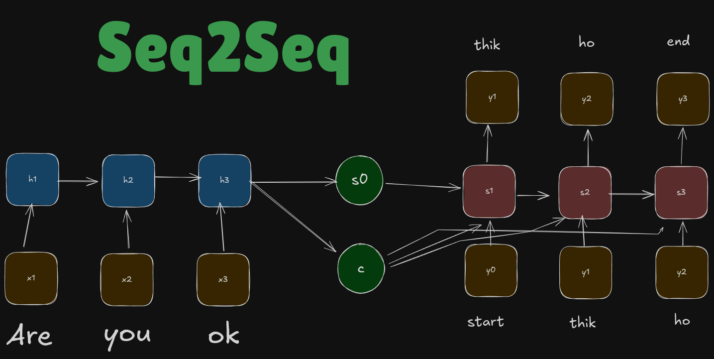
It has two RNNs - Encoder and Decoder. The encoder processes the input and generates a context vector c, which includes all the essential information from the input and also generates an initial decoder state, \(s_0\). The decoder uses this context vector to produce the output sequence step by step, relying on it’s previous outputs and content vector at each step. [We will not go into too much detail as it will take up a lot of blog time]
This kind of solution is good, if we are working with smaller samples, but if we have bigger samples, then the context vector is not able to hold all meaningful information from our encoder part. This is called the bottleneck problem, which is basically the loss of information in the fixed-size context vector!

A sentence like Mohan is a boy, what gender is Mohan? will be all good to pass through the Seq2Seq, but something like

Mohan is a boy. He loves playing football with his friends in the park every evening. His favorite subject in school is mathematics, and he enjoys solving challenging problems. Mohan also helps his younger sister with her homework. On weekends, he visits his grandparents and listens to their stories. What gender is Mohan?

The RNN structure will loose context

Let’s consider two simple explanations why RNNs were losing context —

Explanation 1

RNN forward pass formula is something like —

The next hidden state only depends on the current input and the previous hidden state. That means in the long run, the earlier hidden states are completely ignored and only the previous one is accounted for, thus leading to loss in context.

Explanation 2

The backpropagation method in RNNs or BPTT can give rise to an issue of vanishing gradients. There are three things on which we calculate the loss — \(h, x \space and \space o\) (hidden state, input, and output.

It’s easy to find the gradient of the output but the hidden state is the real problem. Once we unroll the gradients, the chain becomes really big and we get a term with lots of chain rule terms. These gradient values are really small in value and on multiplying them the values of the gradient become negligible.

The gradient diminishes over time, so the network struggles to connect information from earlier time steps to later ones.

mind it, that both of the explanations go hand in hand, not separate. the complete answer is explanation 1 + explanation 2.

Bahadanau Attention

With Attention what we aim to do is, try to create a new context vector at every timestep of the decoder which will give meaning different to each encoded sequence.

What is Attention

Paper Link - Neural Machine Translation by Jointly Learning to Align and Translate

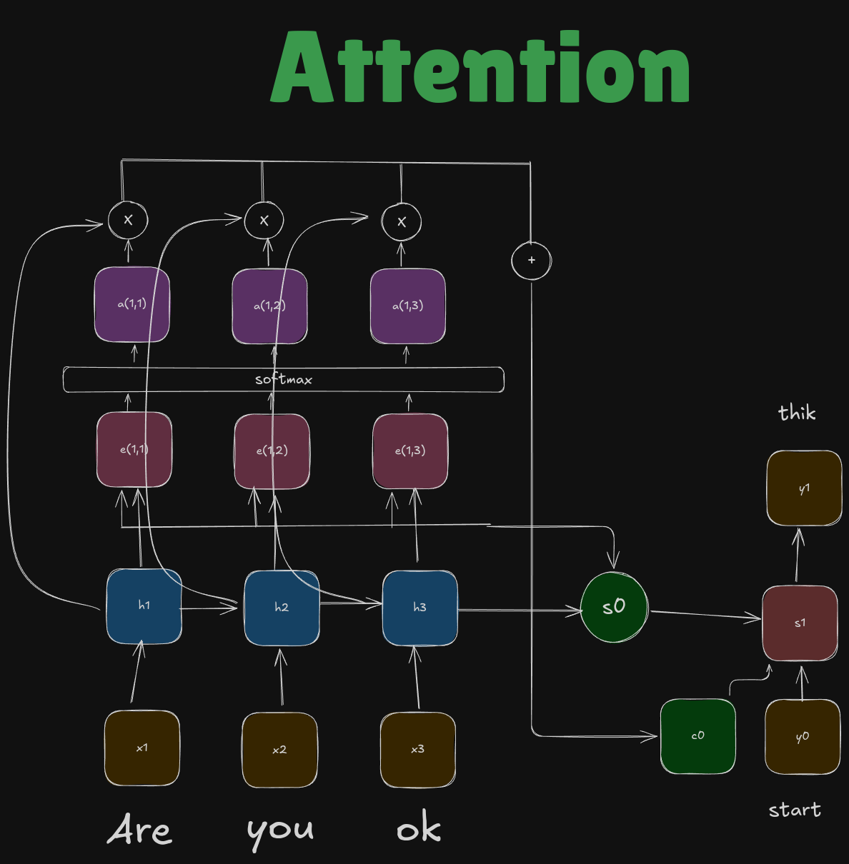
Let’s dissect this at \(t=1\)

E Score

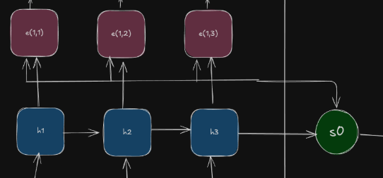
At \(T=t\), we use \(s_{t-1}\) decoder state to find \(e\) . We use a special function \(f\) to compute the value of e.

This function is nothing but a multilayer perception function. It is also called the alignment function.

The numbers are some scalar values that tell us how \(h_1\) is contributing to predict \(s_0\). Since they are scalar values, we must normalize them by applying softmax function.

Attention Score

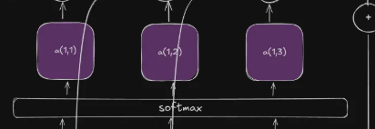
The final result we get after applying the softmax function for each value is called the attention score. They tell us how the hidden state is related to the final \(s_0\) decoder state.

Final Context Vector

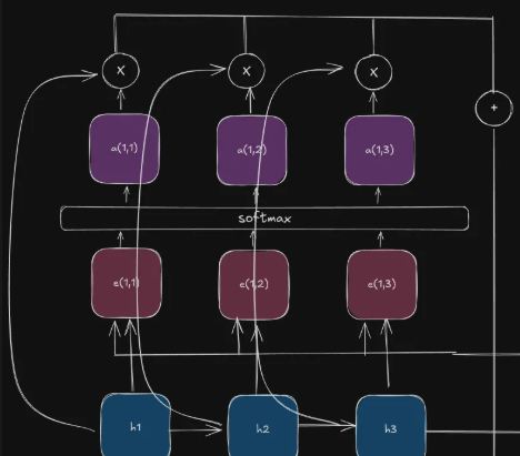
This works in 3 steps.

Step 1

Take the hidden vectors and multiply them with their respective attention weights.

Step 2

Compute the result for each of the attention weights and hidden weights.

Step 3

Add all the results up to get your context vector.

Repeat This

What I did was do the first step. What you’ve to do is to do it for every step, two more times.

Find the \(e, a,c\) for \(t=2,3\) and then consecutively find \(y_2,y_3,y_4\). The method is the same as I have discussed earlier

Exercise: Actually code the whole attention thing using just numpy

Single Head Attention

Now that we know what attention is, let’s try to make an single head attention layer.

Abstract Form of Attention

Let’s try to write attention in the form of variables only!

• Input Vector: \(X\) ( \(N_x\) x \(D_x\))
• Query Vector: q ( \(D_q\)) - It is just the dimension of Query Vector
• Function: \(f\)
• E Score: \(e_i=f(q,X_i)\)
• Attention Score: \(a_i=softmax(e_i)\)
• Output: \(y_i=\sum_ka_kX_k\)

What do we need to change here?

Firstly we will change the function \(f\) to a dot product, instead of doing an MLP operation, but there is a problem. It will give one result only. Additionally, softmax can give rise to a vanishing gradient problem. So we now use a different thing instead of softmax which is a scaled dot product

We also want to calculate all the queries together, and not one by one, thus saving time. So we change our q vector to become a matrix \(Q\) ( \(N_Q \) x \(D_Q\))

New Form of Attention

Let’s try to write attention in the form of variables only!

• Input Vector: X ( \(N_x\) x \(D_x\))
• Query Vector: Q ( \(N_Q \) x \(D_Q\))
• Function: scaled dot product
• E Score: \(E_{i,j}=\frac{q.X_i}{\sqrt{D_q}}\) and \(E=QX^T\)
• Attention Score: \(A=softmax(E,dim=1)\)
• Output: \(y_i=\sum_ka_kX_k\)

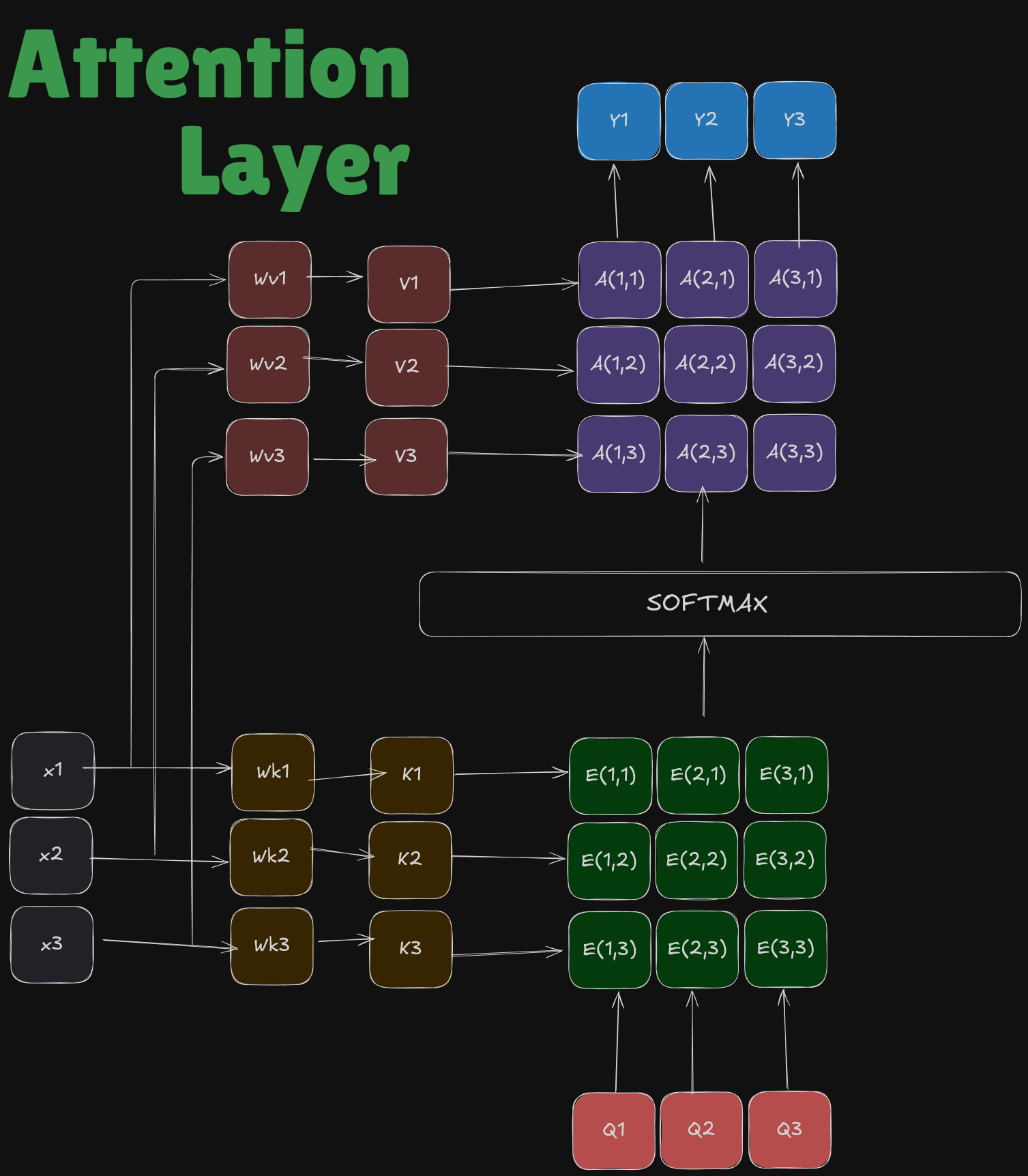
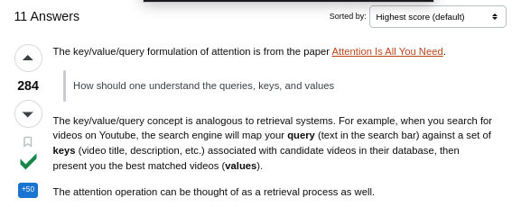
You see two new terms - K and V
If you see you were using the same \(X_1,X_2,X_3\) many times, so we named them in a different way Key and Value. The intuition is very simple from this post I came across long time back!

Here the weights \(W_k ,W_v\) are trainable, and what we try to do in transformers is train them :)

So finally we apply our learnings and end up with the all famous formula of —

Masked Attention

What’s it?

It’s a technique used in models to prevent the model from seeing the future tokens!

Imagine you're trying to predict the next word in a sentence while reading it from left to right. You can only look at the words you've already read, not the ones ahead. This is similar to how masked attention works, where each token can only "look" at previous tokens.

How does it work?

We just add a masking matrix to the attention score!

Now how does the masked matrix look like?