Deepseek R1 for Everyone

a guide into how deepseek r1 works under the hood

We’re gonna discuss how the Deepseek R1 model actually works in detail but with very less math!

The blog will have 3 main parts —

Chain of Thought Reasoning
Reinforcement Learning
GRPO
Distillation

Original Paper Link - DeepSeek-R1: Incentivizing Reasoning Capability in LLMs via...

Chain of Thought Reasoning

This is basically a prompt engineering thing that we apply to the model. We force the model to think rather than just giving us the answer. We add a simple prompt to the user prompt.

Let’s say the user inputs what is the solution of 2+2?, from our side we add a prompt that will be something like please think step by step and explain everything step by step . Let’s now discuss how actually the prompt looked for Deepseek R1 (approximate).

👉

<think>

Understand the Question: Begin by carefully reading and interpreting the question to clarify what is being asked.
Identify Key Components: Break down the question into its essential elements. What are the main concepts or variables involved?
Outline Relevant Information: Consider any formulas, definitions, or prior knowledge that may apply to this problem. What information do I need to solve it?
Step-by-Step Reasoning:
- Clearly articulate each step of your reasoning process.
- Apply logical reasoning to derive conclusions from the information provided.
- If applicable, perform necessary calculations or analyses in a systematic manner.
Summarize Key Points: After completing your reasoning, summarize the main points that are relevant to the question.
Final Answer: Provide a concise answer that directly addresses the question.
</think>
<answer>{{final_answer}}</answer>

This would always give an answer in the following format

<think>{{thoughts}}</think>
<answer>{{final_answer}}</answer>

Let’s see an example run on the question What is the sum of all even numbers from 1 to 100?

👉

<think>
To find the sum of all even numbers from 1 to 100, I first need to identify the even numbers in this range. The even numbers between 1 and 100 are: 2, 4, 6, ..., 100.

These numbers can be expressed as a sequence where each number can be represented as \(2n\), where \(n\) is an integer. The smallest even number is \(2(1) = 2\) and the largest is \(2(50) = 100\).

Now, I can see that there are 50 even numbers in total (from \(n=1\) to \(n=50\)).

To calculate the sum of these even numbers, I can use the formula for the sum of an arithmetic series:
\[
S_n = \frac{n}{2} \times (a + l)
\]
where:

\(S_n\) is the sum,
\(n\) is the number of terms,
\(a\) is the first term,
\(l\) is the last term.

Plugging in the values:

\(n = 50\),
\(a = 2\),
\(l = 100\).

Now substituting these values into the formula:
\[
S_{50} = \frac{50}{2} \times (2 + 100) = 25 \times 102 = 2550.
\]
Therefore, the sum of all even numbers from 1 to 100 is 2550.
</think>
<answer>2550</answer>

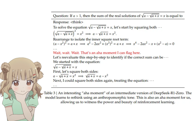
As you can see in the paper itself, the model pauses, and then waits and then, continues to give it a second thought.

Keep in mind CoT is not system prompting! In CoT, it involves appending specific instructions to a query that prompt the model to explain its reasoning step by step (e.g., "Explain your answer step by step”), whereas in system prompting, it involves setting broader parameters for interaction, such as defining the role of the assistant (e.g., "You are a helpful assistant")

Reinforcement Learning

While learning reinforcement learning, we come across two terms — Reward and Policy

Let’s understand them using an example —

Consider the equation \(x^3-9x+7=0\), the solution are three values, but our aim is not to find the correct answers, we also want to find the best way to find the solutions.

Here, we define the method by which we solve as Policy, and we define a score for each method, which judges each policy and assigns a number to it, which we call as Reward.
Below I’ve attached a random Reward v/s Policy graph. Let’s analyze it a bit

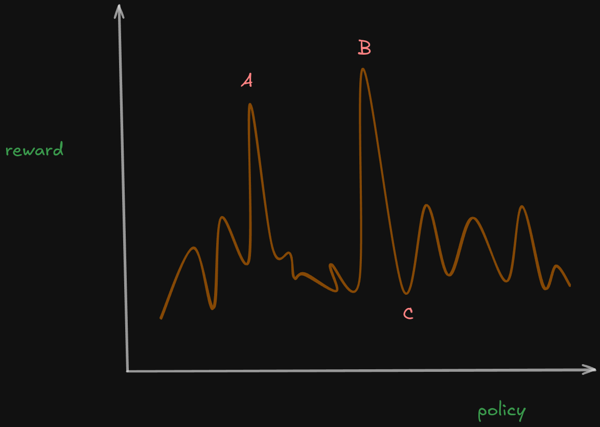
The point C has one of the lowest reward, meaning it will probably be the worst method to solve the equation whereas, points like A and B have one of the highest rewards! The best policy to solve the problem is the policy with the highest reward and is called the Optimal Policy.

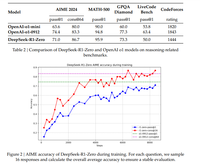
\[optimal\space policy = policy \space with \space reward\space \rarr max[R(P_1),R(P_2),\dots,R(P_n)]\]

In DeepSeek R1, what they do is try to find the best chain of thought to get the answer, they try to run the model on questions (for eg. AIME) and chose the policy which has the highest reward score. In the paper, they reach close to o1 level results using this method of training!

Group Relative Policy Optimization

GRPO is the main thing that sets DeepSeek R1 apart. It tries to find the correct answer without having 0 clue what it is. This basically optimizes the policy and we find the best policy using this. It looks like this —

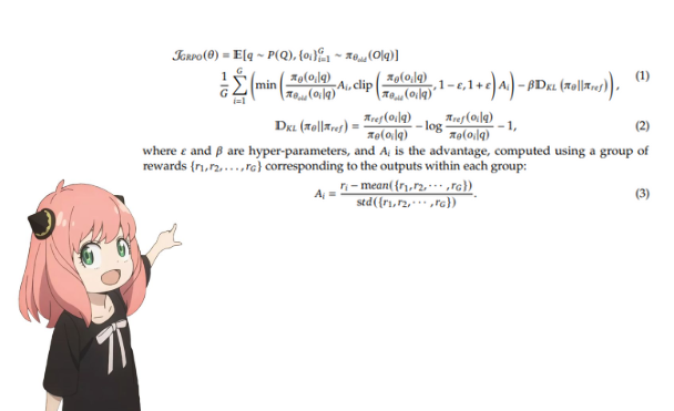
Looks scary right? Let’s dissect this into pieces. The whole equation will be broken into 4 pieces!

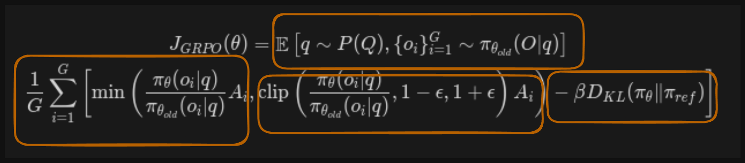
A disclaimer : We are actually finding out the expectation of the whole term based on the Part 1 as input/earlier outputs. The way it is written in the paper is a bit confusing as pointed out by hallerite on Twitter / X. I follow the original formula and assume that you understand that the whole part is under the expectation value.

Part 1

In this part, we basically take the expectation based on the results of earlier policies, and tries to find the average performance over all earlier policies for all inputs and their respective outputs. Think of this as the agent "imagining" all the possible scenarios it might encounter and all the actions it might take. It then evaluates how good or bad those actions are on average.

\[ q \sim P(Q)\]

The input value is q and it ill be sampled from a probablity distribution P(Q). This sets up the task, the agent tries to solve.

\[\{o_i\}_{i=1}^G \sim \pi_{\theta_{old}}(O|q)\]

For every input q, the agent generates G outputs using the earlier old policy. We will be using the earlier policy as the current strategy before the update happens for the newer policy.

Part 2

Imagine you're trying to improve your cooking skills. You don't want to completely change your recipe (policy) all at once because it might turn out terrible. Instead, you make small adjustments and only keep the changes that actually make the dish better. This part ensures exactly that!

\[ \frac{\pi_\theta(o_i|q)}{\pi_{\theta_{old}}(o_i|q)}\]

This ratio measures how much likely the new policy is gonna take the output as compared to the older policy. It basically ensures that the new policy doesn’t deviate much from the older policy, this leads to stable training!

\[A_i=\frac{r_i-mean(r_1,r_2,...,r_G)}{std(r_1,r_2,...,r_G)}\]

This \(A_i\) is called the advantage function and it measures how much better/worse the current output is compares to average of all the earlier outputs.

Finally we find the min so that if the values of outputs that will have very high advantage, they don’t get updated which will lead to loss in stability.

Part 3

Think of this as putting guardrails on your policy updates. You don't want to take huge leaps that might lead to bad outcomes; instead, you take small, controlled steps. The clipping function actually just clips the value to some extent and doesn’t let it cross a threshold!

\[\text{clip}\left( \frac{\pi_\theta(o_i|q)}{\pi_{\theta_{old}}(o_i|q)}, 1 - \epsilon, 1 + \epsilon \right)\]

The clip function restricts the ratio to be in the range of \([1-\epsilon,1+\epsilon]\), where \(\epsilon\) is a very small number, and it keeps the value of the ratio in check. Clipping prevents the new policy from making drastic changes, which could destabilize training.

Part 4

Imagine you're learning to drive. You have a driving instructor (the reference policy) who gives you good advice. The KL divergence term ensures that you don't completely ignore their advice and do something reckless.

\[- \beta D_{KL}(\pi_\theta \| \pi_{ref})\]

The KL divergence measures how different both the policies are to each other, it keeps in check so that the new policy doesn’t stray too far from the reference policy.

More about KL Divergence

The beta term is just a weight factor which controls how much the KL divergence term influences the overall objective.

Summary

The expectation part ensures the objective considers all possible scenarios.
The min and clip parts ensure that updates are stable and incremental.
The KL divergence part ensures the policy stays close to a reference policy.

GRPO balances exploration (trying new actions) and exploitation (sticking to what works). It ensures that the policy improves without making drastic changes that could lead to poor performance.

Distillation

I have taught distillation in detail in my another blog, please visit it to learn all about distillation!

Link to the blog - Enhance Your Model - 1 [Week 9]

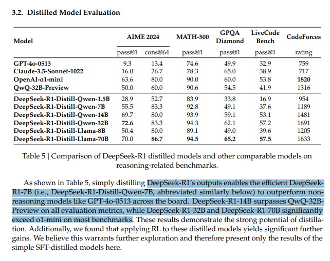
The distilled form of DeepSeek R1 outperforms many SOTA models even though it’s at much lesser parameters!

A very important section of the model itself is the DeepSeek v3 model, which has been beautifully explained by Himanshu, check out his blog on the same —

Deepseek-v3 101

Reference Material Used

DeepSeek-R1: Incentivizing Reasoning Capability in LLMs via... (Overall)