Enhance Your Model - 1 [Week 9]

You built a model. Really nice, but how to make it better? How to make it work seamlessly, so that it solves the issues that it faces in the first place. Exploding gradients, unstable learning rate? We try to solve each of them

This first part of the blog series will contain 4 topics

• LoRA
• Knowledge Distillation in Neural Networks
• Early Stopping
• Gradient Clipping

Low-Rank Adaptation (LoRA)

Paper Link - LoRA: Low-Rank Adaptation of Large Language Models

Short Intro to Finetuning

Let’s consider a neural network, which we want to build to classify cats and dogs.

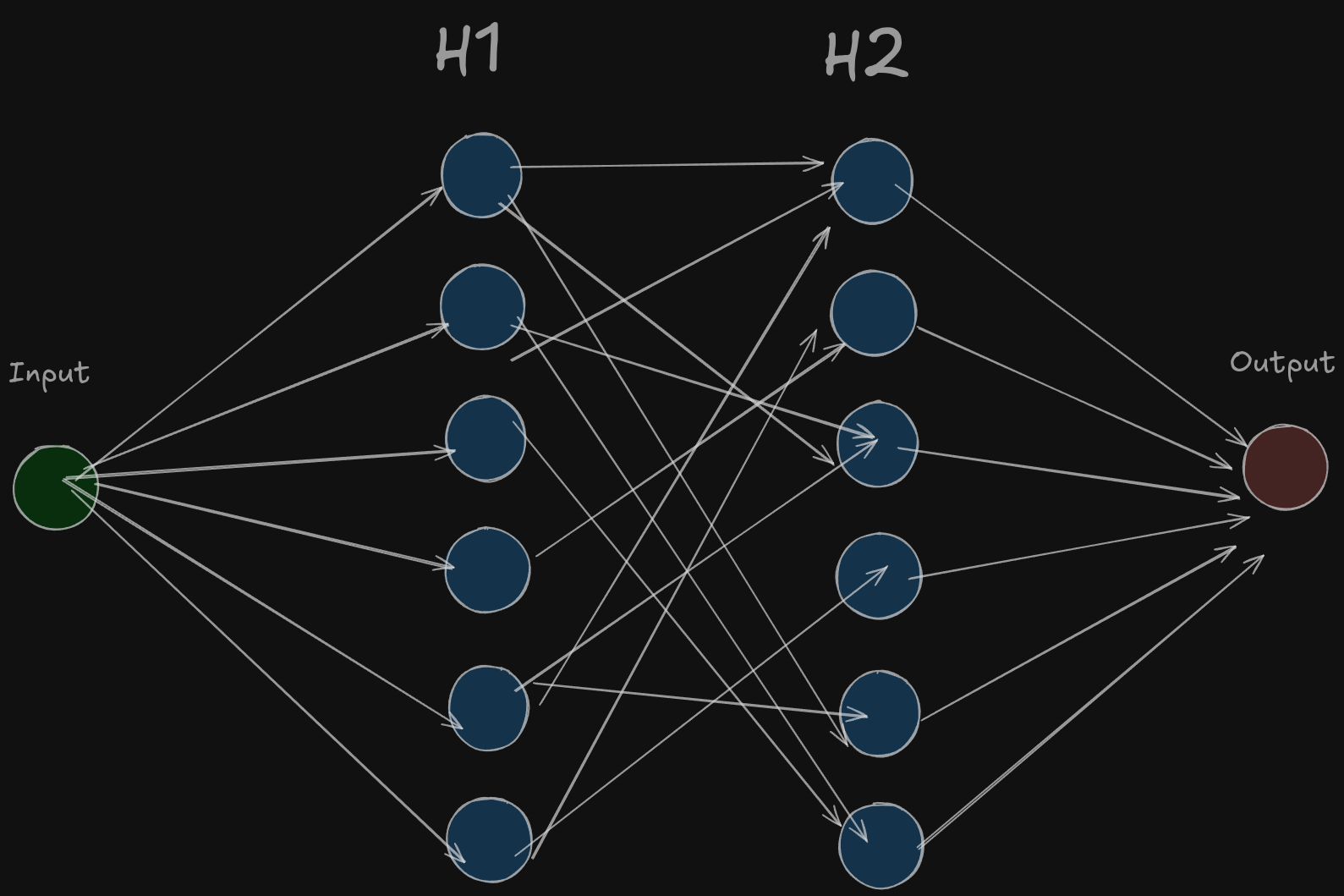
Now, to build an intricate model like the above one and train it from scratch, we will be needing a lot of resources, so what we do is we load the weights of a pretrained network like the above one, and then we construct a new layer that segregates the learning of earlier detailed model into two classes of cats and dogs. We freeze the weights of the earlier model to retain the learning and we just train the last layer of H3

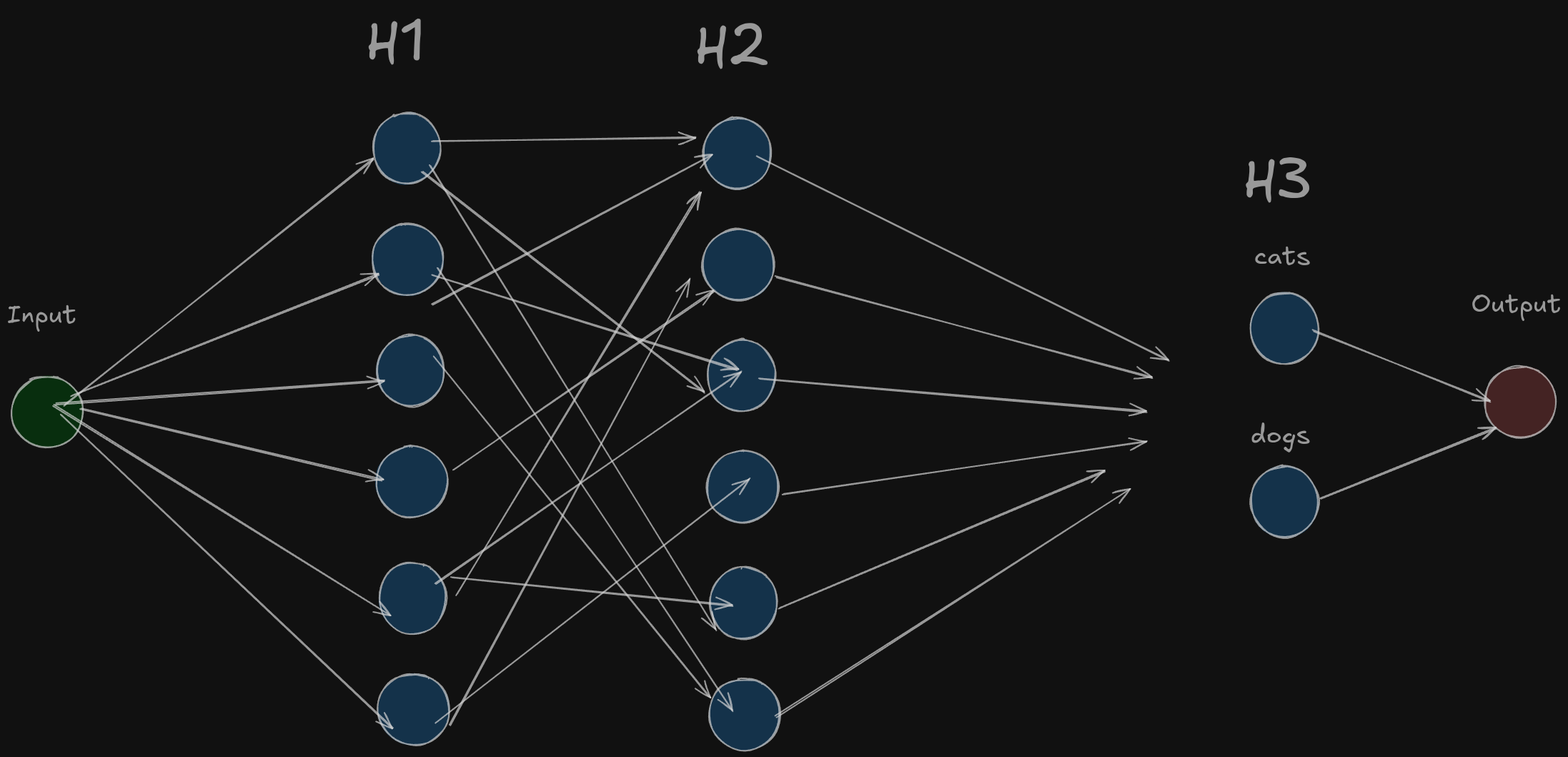
By this method, we use earlier knowledge and save a lot of training time. This kind of finetuning is called Classification Fine-tuning. There are other different types too, but we’ll not go in detail as e intend to just learn LoRA now.

What’s a major problem with finetuning is, even if we train just the last layer or even any other layer, it’s huge in size and processes the earlier stuff as well, which is computationally very expensive. Additionally, if we are using many models, loading weights for each of them individually will be very time inefficient and expensive!

To fix this, we introduce LoRA!!!

How does it work?

Usually we would have used the pre-trained weights in the neural network. Let’s analyse how many params that would take.

Imagine the dimensions of the pre-trained weights to be \(d=1000 \space \& \space k=6000\)

Then the number of params would be —

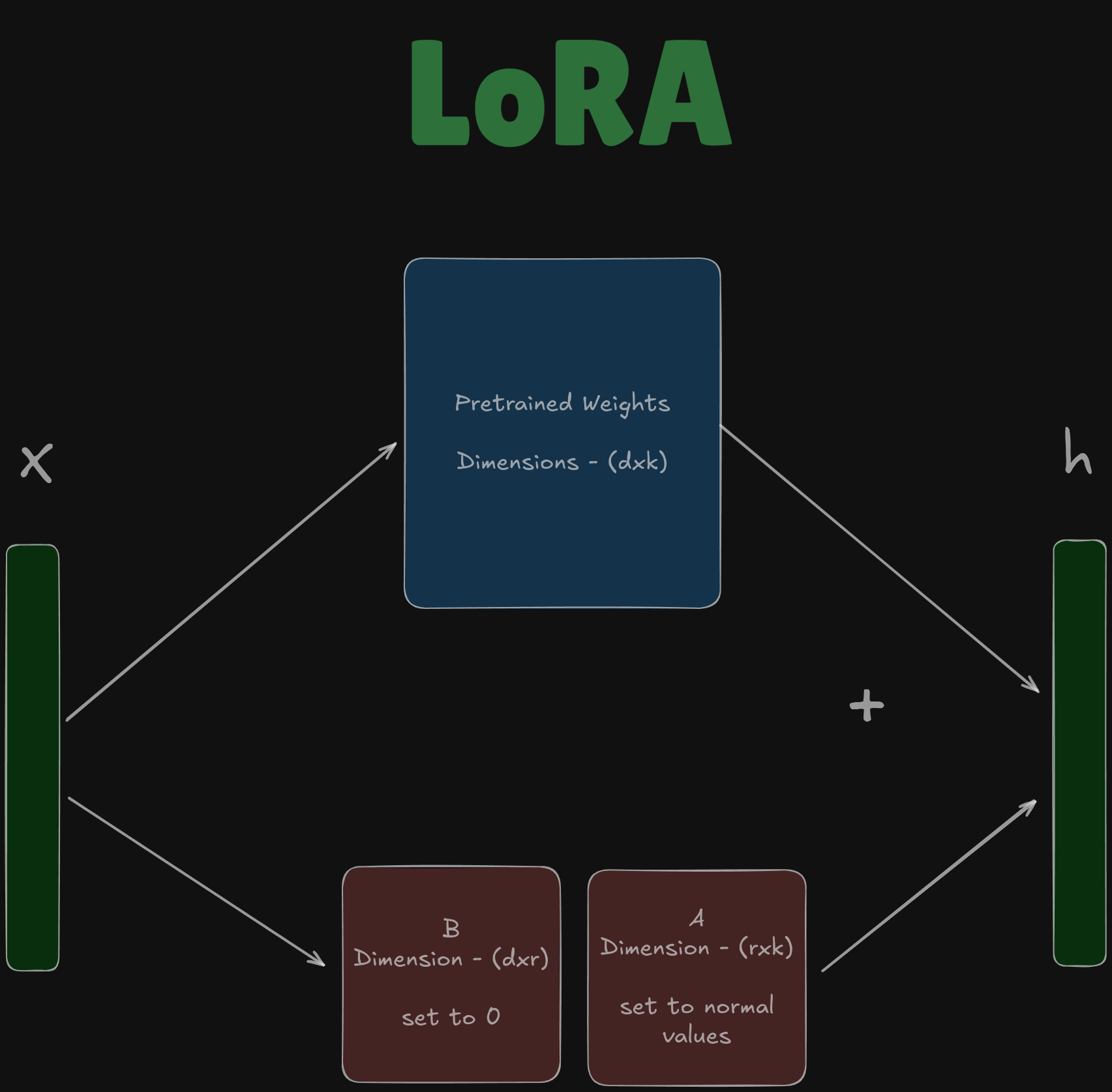
Now let’s calculate in the case of LoRA,

You notice a term \(r\) in the dimensions of B and A, we define r as —

meaning, r is chosen as a very very small value, in our case let it be 2.

We define two matrices —

1. A : dimensions are \((r,k)=(2,6000)\), and every value is randomized according to the normal distribution
2. B : dimensions are \((d,r)=(1000,2)\), and every value is set to 0 at first.

What’s the number of params in this case?

We literally shortened the number of parameters to around 0.2% of the original parameters.

You might wonder, why is this ever working?

Why does it work?

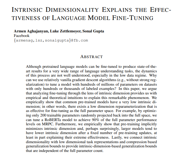
This paper discusses something that makes LoRA work, despite such low amounts of parameters.

This tells us that even if the weights of a pretrained model are randomly projected into a smaller space, they still can learn all the features from the pre-trained weights, thus confirming that pre-trained models have indeed a low intrinsic dimension. We can remove the extra dimensions and still retain all the performance of the earlier matrix.

Exercise : Build any finetuned small model that classifies a cat and a dog, then apply LoRA to it. Compare the difference in performance and difference in parameters.

---

Knowledge Distillation in Neural Networks

Paper Link - Distilling the Knowledge in a Neural Network

Softmax in Detail

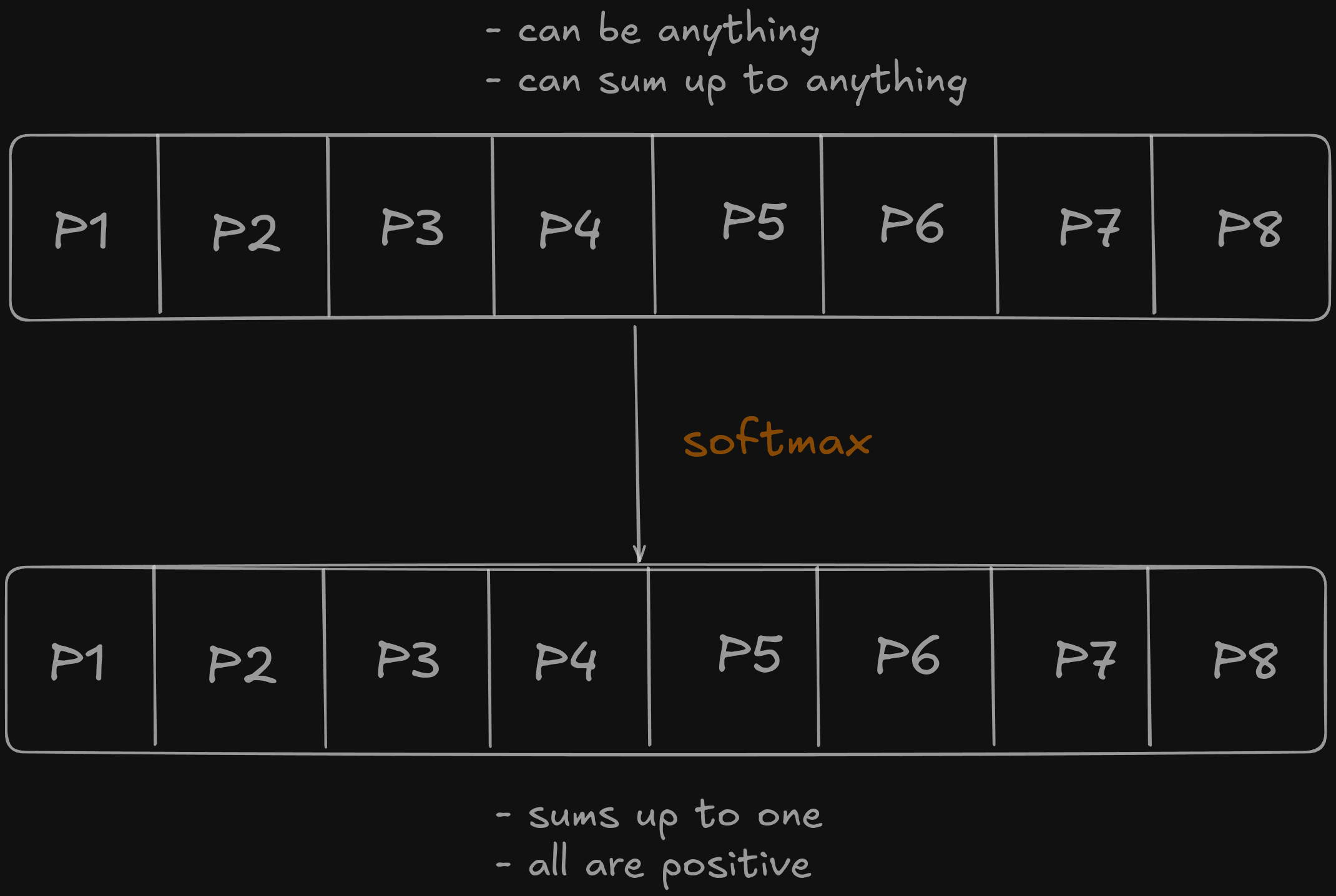
The last layer of many neural networks is a softmax function, which is essentially —

But have you ever wondered why do we even use this function. Why do we do this \(e^x \) operation and normalize it over every value.

The answer is simple — We want a probability distribution! Every value should be positive (reason for \(e^x\)) and all of them should sum up to 1 (reason for normalization)

But a follow up question might be why do we even want the final output to be a probability distribution?

It’s because our final output always gives an answer is the probability of each class happening, and my ground truth labels, with which we will compare the values to find out loss, are all one-hot encoded vectors.
One-hot encoded vectors are a kind of probability distribution itself as it sums up to one and is positive, but only one value gets all of the values, hence we try to make the output from our neural network a probability distribution as well.

Problems with Softmax

The loss function we generally use in most cases is cross entropy loss, which is —

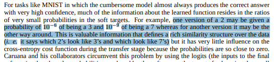
But a huge problem with this is that softmax pushes the higher values to a much higher value while not giving any preference to lower values. As discussed in the paper, they tell ho a picture of 2 may be closer to 3 rather than to 7, and normal softmax will not capture that! Softmax hides relative similarity between other classes, and this is a very important information.

How to Solve this?

We need to retain the feel on the relative similarities between classes while we are still using softmax, as we need the probability distribution.

The authors decided to do one thing — let’s make the logits smaller, before doing the exp operation . This would smoother the graph and give closer values to similar classes! This removes the concept of a single value having a huge spike in value

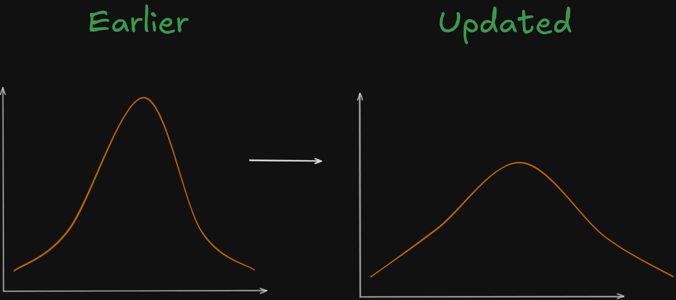
Every logit was divided by a number \(T\), this number is nothing but called the Temperature. Higher the temperature, flatter and smoother the curve is. The updated formula became —

In reality, you are supposed to find the value of T by experimentation after doing several runs.

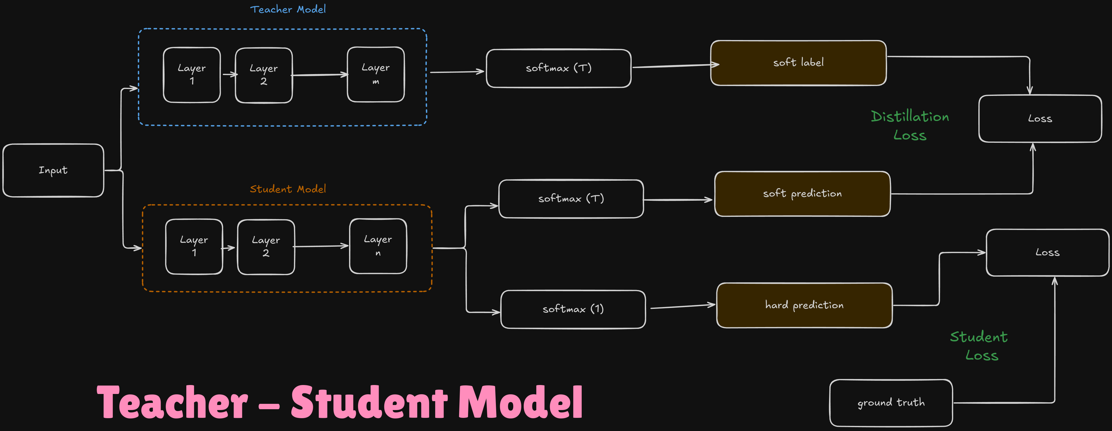
Teacher - Student Model

Teacher Model

It is a large and complex neural network that has been trained on a large dataset, and has a complex structure in itself. This teacher is like the master which makes highly accurate predictions. But since it’s having much more parameters in reality, it is computationally expensive to use in real life!

Student Model

It is basically a smaller and efficient neural network with much fewer layers than that of the teacher. Our objective is to train this model to copy the behaviour of the teacher model, thereby achieving almost similar performance with lesser computational resources!

Imagine the teacher model is a seasoned professor who has a deep understanding of a subject. The student is a new learner trying to grasp the subject.

What are the terms?

1. Soft Labels - They represent the teacher's predictions in a probabilistic form. We use the softmax function with temp>1 here on the teacher model
2. Soft Predictions - They represent the student's predictions in a probabilistic form. We use the softmax function with temp>1 here on the student model
3. Hard Predictions - They represent the student's final predictions. We use the softmax function with temp=1 here on the student model.
4. Ground Truth - Also called hard labels, these are the actual answers with which we will be comparing out results (usually they are stored in one-hot encoded form.

Consider that the professor provides detailed explanations (soft labels) that capture nuances, while the student also has access to textbooks (hard labels) for direct learning.

Loss Functions

We come across two loss here —

1. Distillation Loss

This loss term uses the soft labels from the teacher and the soft predictions from the student. It encourages the student to mimic the teacher's probabilistic outputs. The loss function here is basically the KL Divergence, which measures how one probability distribution diverges from a second.

The distillation loss encourages the student model to produce probability distributions that are similar to those of the teacher model. This is beneficial because the teacher model's outputs might contain additional information about the relationships between classes, which can help the student model learn more effectively.

1. Student Loss

The student loss ensures that the student model also learns directly from the ground truth labels. This is typically computed using the cross-entropy loss, which measures the difference between the predicted probability distribution and the true distribution.

This is crucial for maintaining the model's ability to perform well on the actual task, not just mimic the teacher.

1. Total Loss

The total loss is a weighted sum of the distillation loss and the student loss:

---

Early Stopping

What’s the problem?

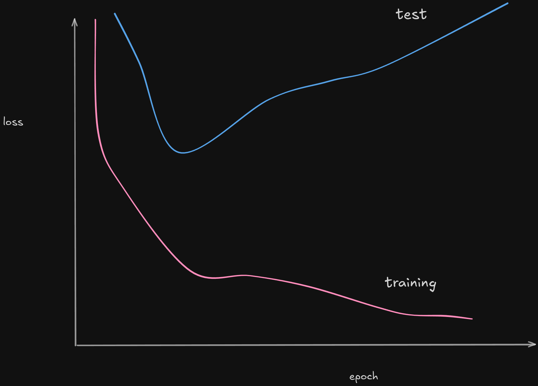
Now let’s say you train a model on 50000 epochs, in most cases it will overfit heavily. While the model might perform great on the training set (showing better performance), when introduced to new data in the test set, it will fail to perform upto the mark and give bad results!

How to solve it then?

We introduce something called Early Stopping!

In the training scenario, we usually have three sets of data

• Training Data
• Validation Data
• Test Data

What we do with the validation data is we try to monitor the loss on the validation set while we are running the training with the training data. What purpose does it serve?