Transformers [Week 2]
a deep dive into transformers and a visual guide into how it works
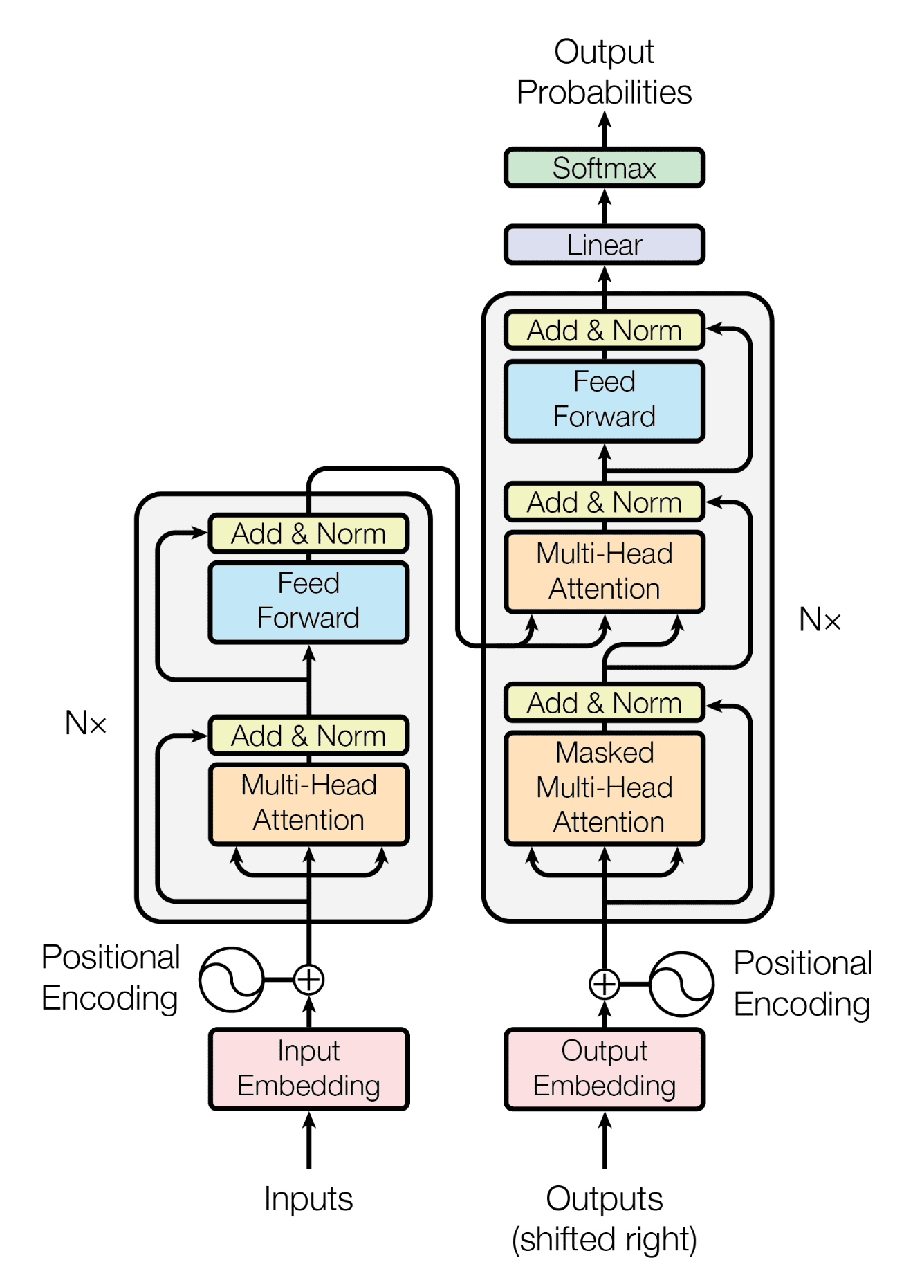
We all have seen this image from the Attention is All We Need paper. Looks scary, right? Let’s try to understand how this actually works using one single example and try to make this journey as simple as possible!
Part 1 (Preprocessing)
Dataset
First we must have a dataset, with which we will be working throughout our journey. For example, the dataset used in GPT3 is 570GB! We can’t obviously use that here as an example, so let’s make a short dataset with only 3 sentences

This will be our Dataset ( some lines from my favorite TV Show ~ The Big Bang Theory. Extra points if you guess who told them :D )
Vocabulary
First let’s break down the dataset into individual words, called as tokens.
dataset = [
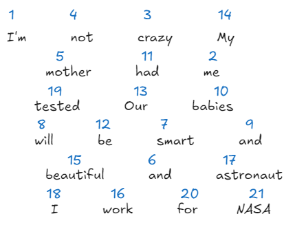
"I'm", "not", "crazy", "My", "mother", "had", "me", "tested",
"Our", "babies", "will", "be", "smart", "and", "beautiful",
"I'm", "an", "astronaut", "I", "work", "for", "NASA"
]We must build our vocabulary now! It’s nothing but the set of unique words in the dataset
The vocab dataset will look something like
vocab = [
    "I'm", "not", "crazy", "My", "mother", "had", "me", "tested",
    "Our", "babies", "will", "be", "smart", "and", "beautiful",
    "an", "astronaut", "I", "work", "for", "NASA"
]
We can easily find the vocab size by :
Encoding
Let’s assign a unique number to each of the word in vocab
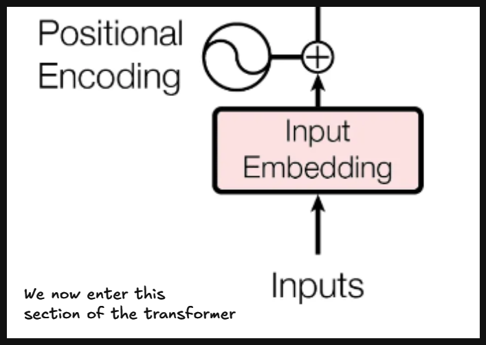
This is all the preprocessing of data we will be needing, now we will delve deep into the transformer architecture itself!
Part 2 (Encoder Embedding)
Embedding
We now need to select a specific part from our dataset. Let’s choose
“Our babies will be smart and”
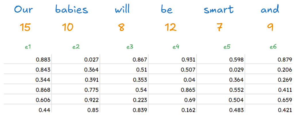
We have selected our input, and we need to find an embedding vector for it.
We will be using a 6-dimensional embedding vector. The values of such vectors are always between 0 and 1 and will be defined at random at the beginning of our journey. We will be updating them as we go on
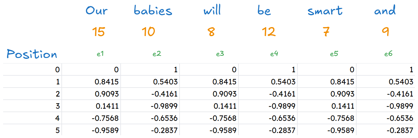
Positional Embedding
Now we find the positional embeddings for our input text. The formulas of that are(first formula for even positions, second formula for odd positions) :
Let’s find the positional embedding for one of the words (Our) :
| i | e1 | position | p1 |
| 0 | 0.883 | even | 0 |
| 1 | 0.843 | odd | 0.8415 |
| 2 | 0.344 | even | 0.9093 |
| 3 | 0.868 | odd | 0.1411 |
| 4 | 0.606 | even | -0.7568 |
| 5 | 0.440 | odd | -0.9589 |
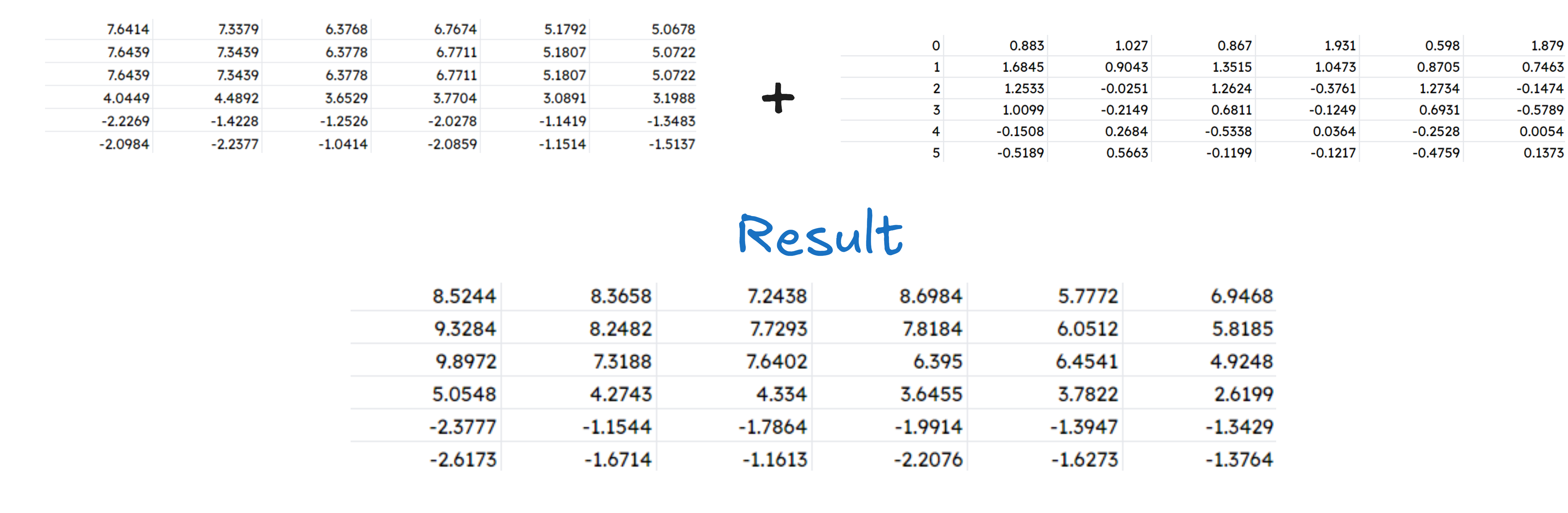
Finally we can find all the positional embeddings of our words to be :
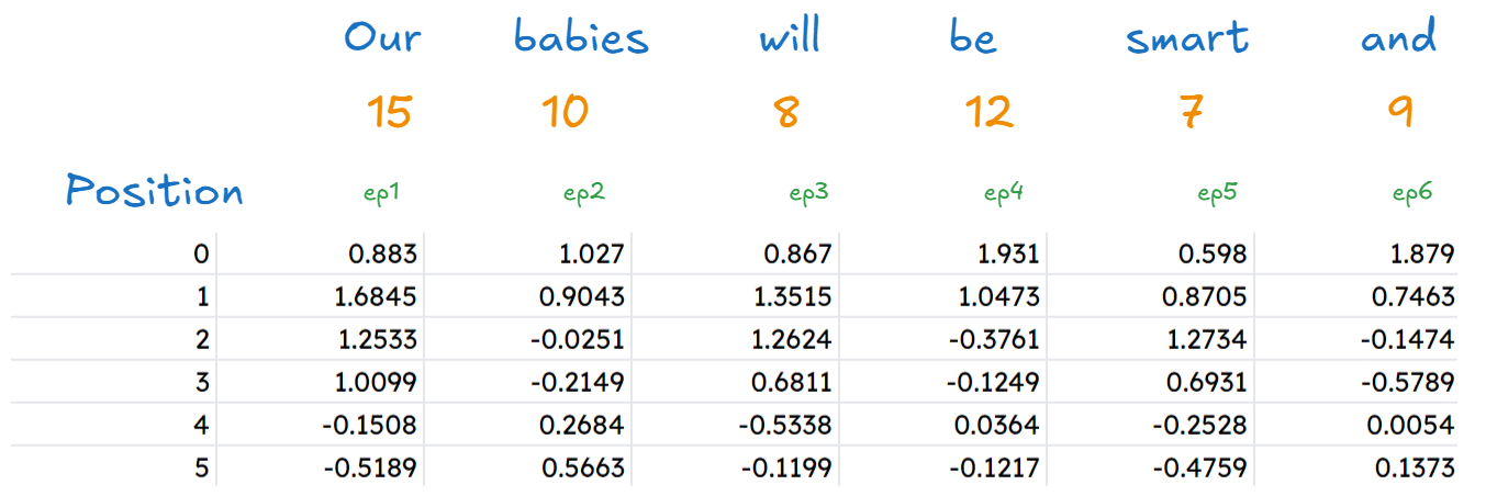
Add both of them
The final step of part 2 is adding both of them. Final result comes out to be :
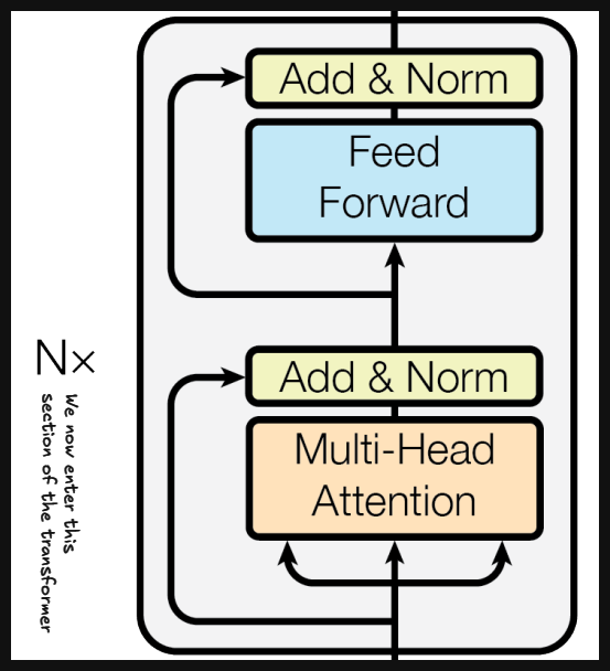
Part 3 (Encoder)
Attention
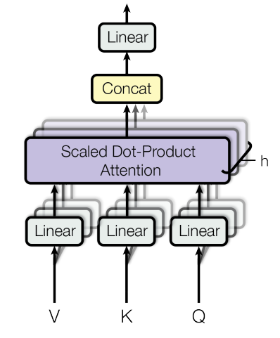
A multihead attention is nothing but many single head attentions combined together. It is our decision how many heads we want to us. Let’s just focus on single head attentions for now!
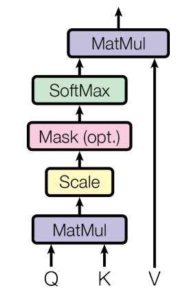
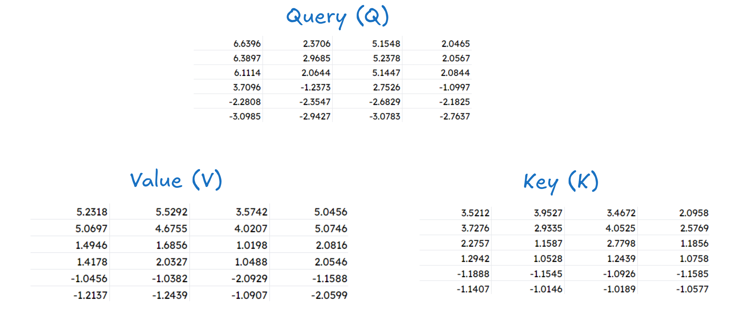
We can see 3 terms here : Query(Q) , Key(K) and Value(V)
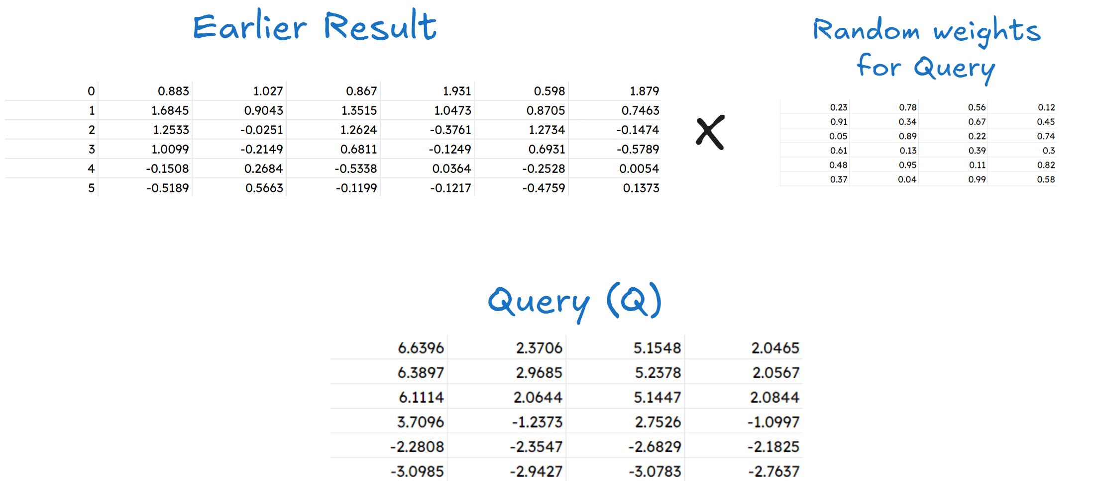
Finding out Q, K and V
We get the respective values of all these by multiplying a weight matrix (must be different from the earlier weight matrix) with the earlier result matrix. Let’s compute Query!
The set of the weight matrix must have same number of rows as the columns of the matrix result from earlier part. This weight matrix has random values from 0 to 1.
Similarly we can find the values for Key and Value as well (I will skip showing it as it will make the blog unnecessarily long!). The values are :
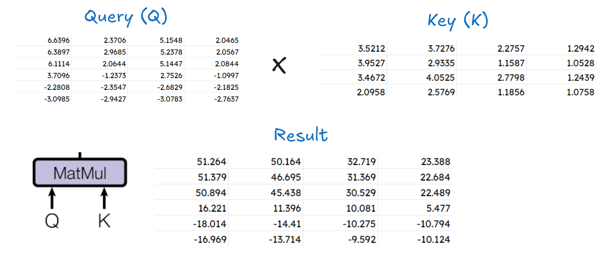
Calculating the attention
First step is \(Q.K^T\) (MatMul section)
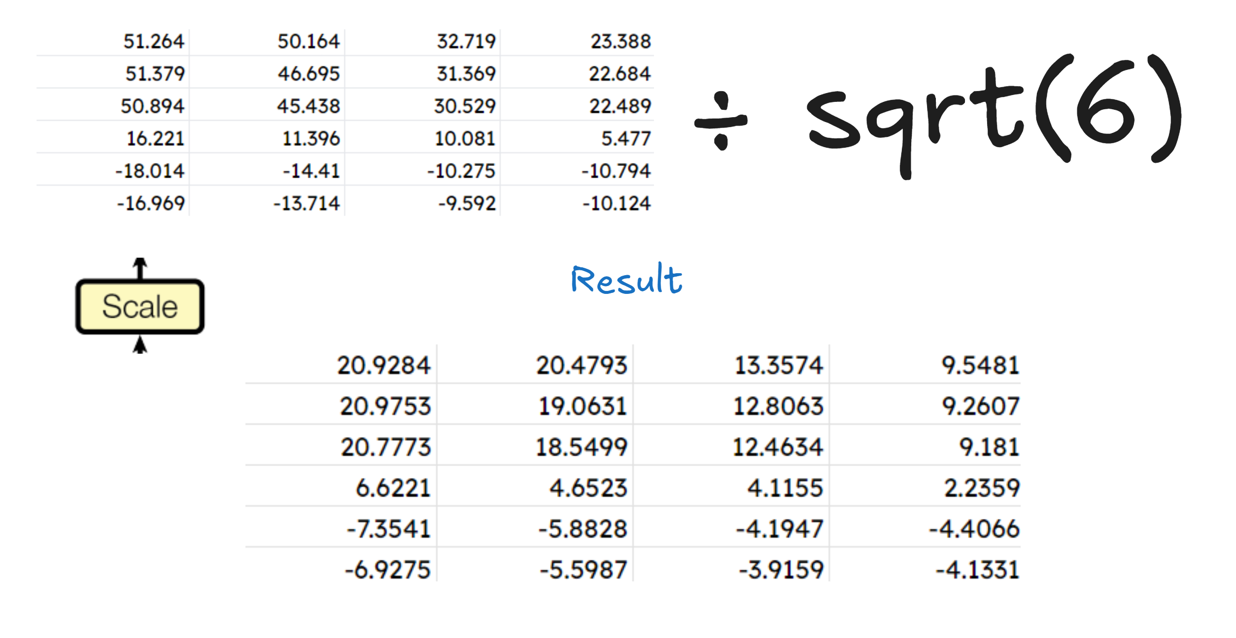
Now, we scale it. By scaling, we want to divide each of the numbers by \(\sqrt{d_k}\) , which is the dimension of our embedding vector.
Now since masking is optional here, we will skip masking for our tutorial(we’ll be covering it later anyways)
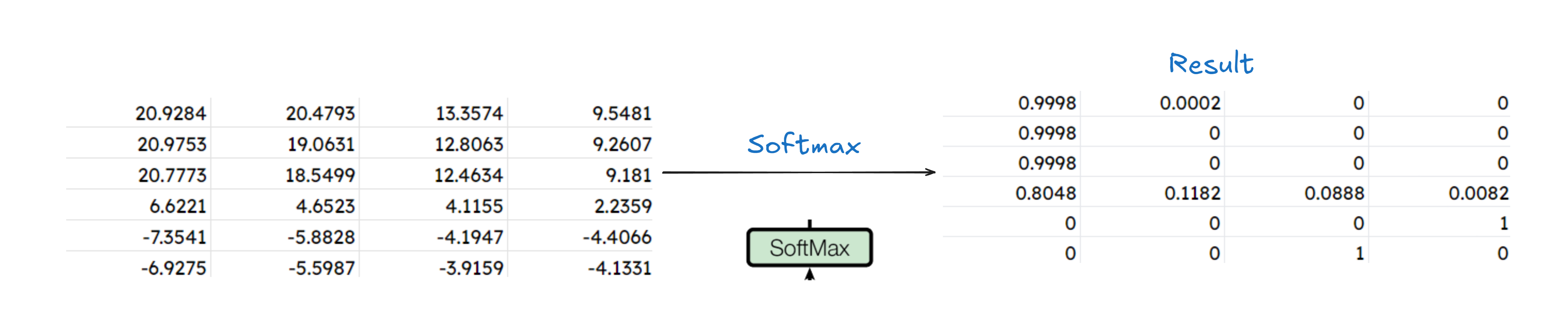
Now we apply softmax to this. Formula for it
Finally we need to apply MatMul operation on our result with the initial Value(V), to get the final output from a single head attention block.
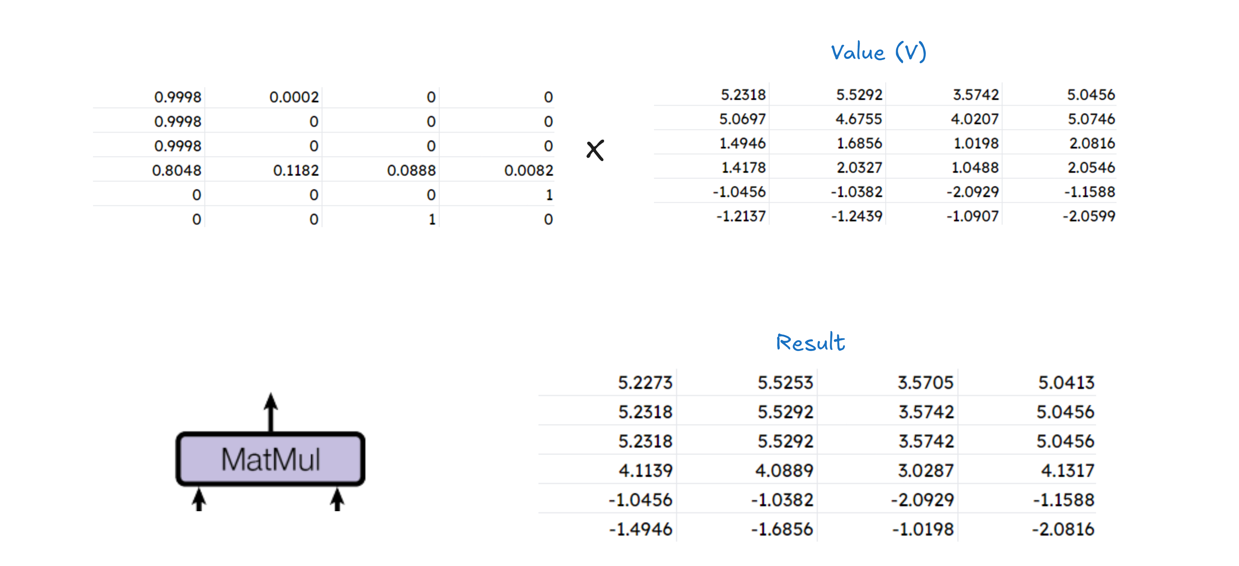
In the paper, attention is mentioned as :
We literally just solved this scary equation using nothing but simple mathematics :D
We now have calculated single-head attention, while multi-head attention is many single head attentions combined together. It looks like :
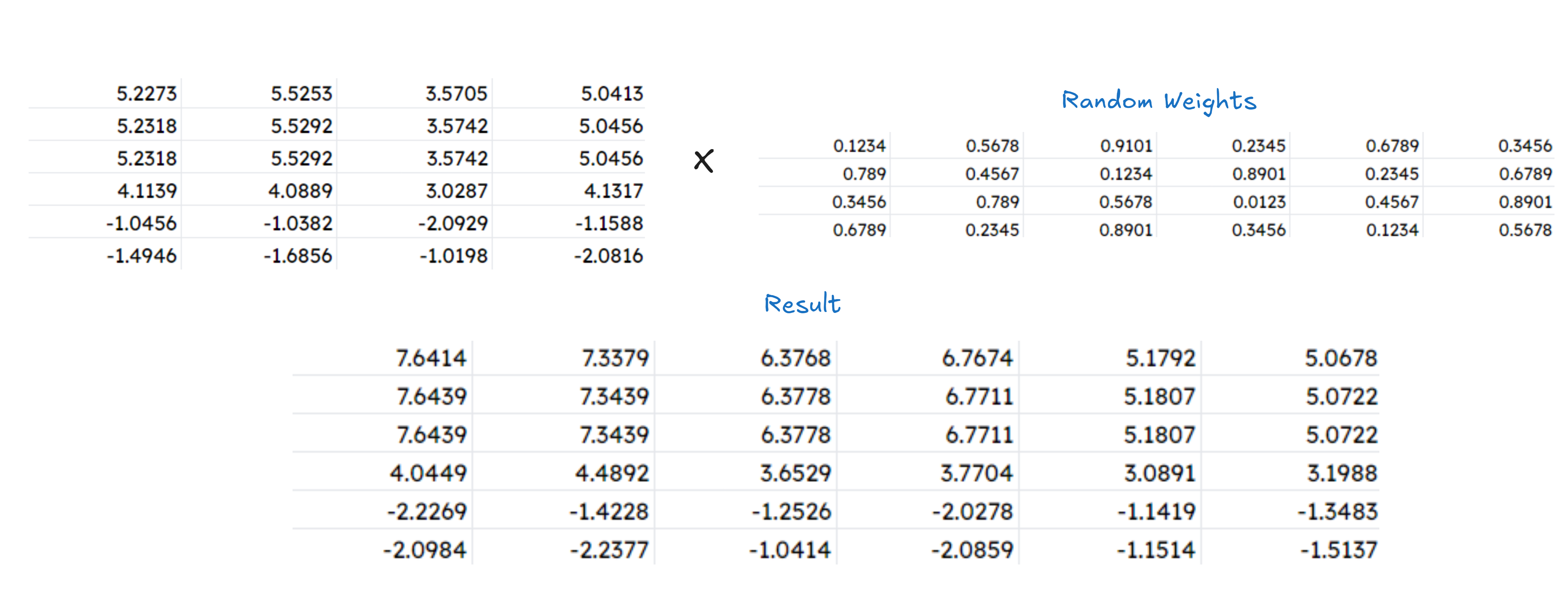
Once we get the results from all such individual single head attentions, they will be concatenated, and the final result is transformed by multiplying it with a weight matrix, with random values. [not writing again, as I’ve shown the process many times above!]
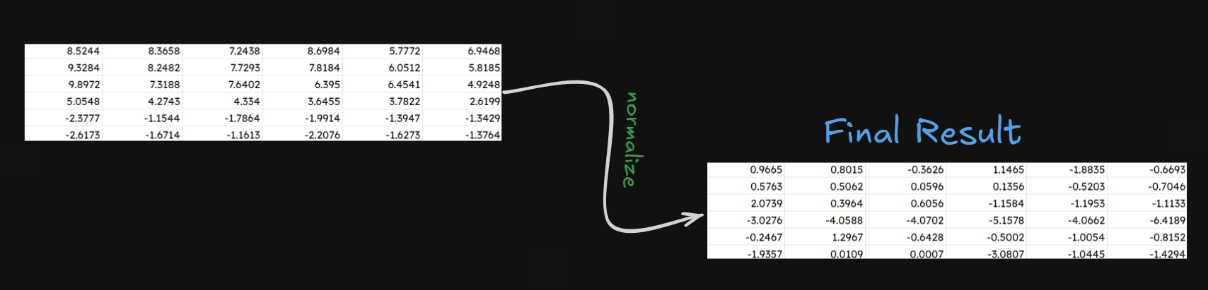
Even if we have a single-head attention or multi-head, we must normalize it before declaring it to be the final output.
This final result is our output of the attention!
Add and Norm
We will add the output of our attention layer to the \(word\space embedding+positional\space embedding\) matrix.
Now we normalize the matrix, by finding row wise mean and row wise standard deviation and normalizing them by this formula
The mean and standard deviation comes out to be :
| Row | Mean | Standard Deviation |
| Row 1 | 7.5927 | 0.9649 |
| Row 2 | 7.6590 | 1.1640 |
| Row 3 | 6.7033 | 1.5519 |
| Row 4 | 3.9250 | 0.8729 |
| Row 5 | -1.5795 | 0.3229 |
| Row 6 | -1.6760 | 0.4875 |
After applying our formula, we reach the final result!
Feed Forward Network
In the feed forward network, we just use a series of Linear and ReLU layers next to each other.
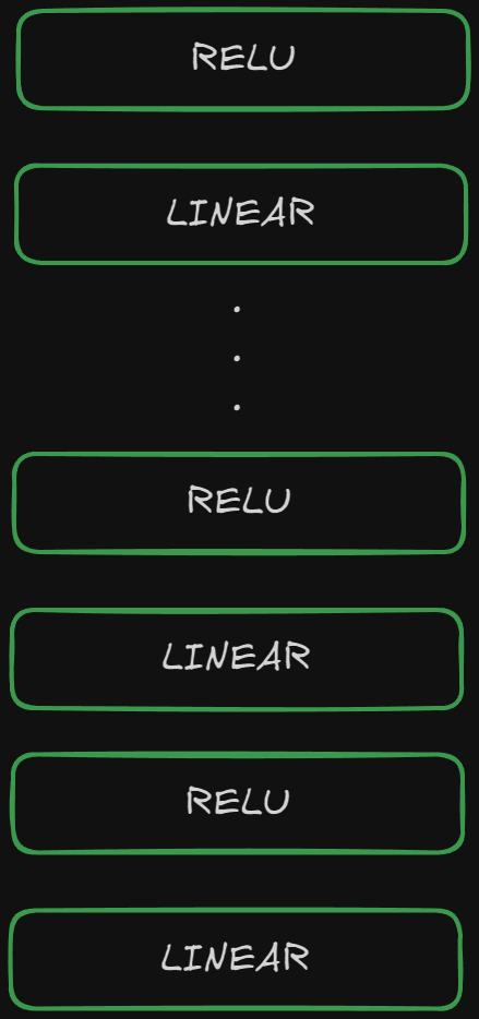
But we will be calculating only one linear and one relu layer for this blog!
Linear Layer
We start by multiplying our last calculated matrix with a random set of weights matrix, followed by adding it to a matrix of bias, which is also made of random values.
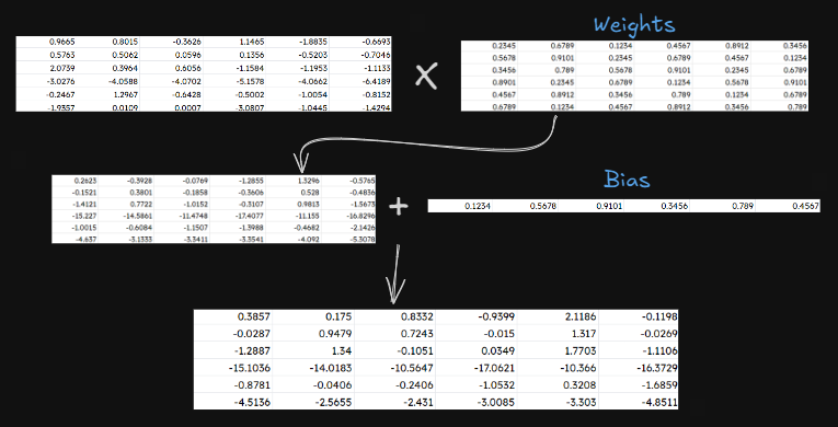
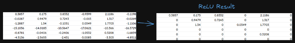
ReLU Layer
Now we just apply ReLU layer on it, which is :
Add and Norm(again)
We’ll just add the earlier result from attention part with the result from this feed forward result. then normalize it with Mean and Standard Deviation to get the final result for the Encoder part!
I will not show the calculation for this, as we have already covered this
Part 4 (Decoder Embedding)
We have successfully finished the encoding part, now we move on to the decoding part. We will be skipping most parts of the decoder as they have been already covered in the encoder part in details. Calculating the rest of the results is left as an exercise for the reader :D
Output Embedding
What would be the input for the decoder? Let’s answer this :