Optimizers [Week 3]
a deep dive into optimizers and a journey through time
In deep learning, an optimizer is a crucial element that fine-tunes a neural network’s parameters during training. Its primary role is to minimize the model’s error or loss function, enhancing performance.
Optimizers facilitate the learning process of a neural network by iteratively updating the weights and biases received from the earlier data. We will discovering optimizers by taking a small road trip down the history of optimizers and slowly inventing newer and more advanced optimizers!
Premise
What we are trying to do here is nothing but to minimize the loss function of any model. Our objective is to find a set of values for which the value of the loss function is to be minimum
We will be employing several methods to do so, while trying to make our optimizers better and better.
Approach 1 - Random Search
Logic
First and the most obvious solution is generate random parameters and find loss with that set of values, if the loss is lesser than our minimum loss, we will keep updating it! After few thousand iterations, we will find our optimum set of parameters
Code
min_loss=float("inf")
for n in range(10000):
	W=np.random.randn(10,2073)*0.0001 #random parameters
	loss=L(X_train,Y_train,W) #calculate the loss
	if loss<min_loss:
		min_loss=loss
		min_W=W
	print(f"Attempt {n} | Loss - {loss} | MinLoss - {min_loss}")
If we actually run this, it will give us an accuracy of around 16.3% (which is not actually that bad, considering it’s just random numbers.
Our first approach is not that good in terms of actually finding the optimum parameters, let’s try a more intuitive approach!
Approach 2 - Numeric Gradient
Logic
What if we try to follow the slope of the curve of the loss function? In a 1-D case, the formula of the derivative is nothing but :
The slope of any curve is nothing but it’s dot product of its direction with the gradient. Let’s take an example table of weights and find their slopes.
| W | W+h | dW |
|---|---|---|
| 0.34 | 0.34+0.0001 | ? |
| -1.11 | . | ? |
| 0.78 | . | ? |
| 0.12 | . | ? |
| 0.55 | . | ? |
| …….. | ……… | …… |
| Loss : 1.25347 | Loss : 1.25322 |
| W | W+h | dW |
|---|---|---|
| 0.34 | 0.34+0.0001 | -2.5 |
| -1.11 | . | ? |
| 0.78 | . | ? |
| 0.12 | . | ? |
| 0.55 | . | ? |
| …….. | ……… | …… |
| Loss : 1.25347 | Loss : 1.25353 |
Let’s find the rest of the values like this
| W | W+h | dW |
|---|---|---|
| 0.34 | 0.34 | -2.5 |
| -1.11 | -1.11 | 0.6 |
| 0.78 | 0.78+0.0001 | 0 |
| 0.12 | . | ? |
| 0.55 | . | ? |
| …….. | ……… | …… |
| Loss : 1.25347 | Loss : 1.25347 |
What’s the problem with this method?
We can go on and on with this method, but it’s evident - It’s too slow, and you can see it’s very tedious to calculate even in 1 dimension, imagine doing this over multiple dimensions. It also tends to approximate the descent by a huge amount! So let’s try to think more intuitively for this.
Approach 3 - Analytic Gradient
Logic
We can realize that loss is nothing but a function of W.
We need to find where the gradient of the loss function is minimum w.r.t to its weights to find out our optimal parameters. Our goal is to minimize \(\nabla_W\space L\) .
| W | dW |
|---|---|
| 0.34 | -2.5 |
| -1.11 | 0.6 |
| 0.78 | 0 |
| 0.12 | 0.2 |
| 0.55 | 0.7 |
| …….. | …… |
| Loss : 1.25347 |
Why is it better?
This method is quite direct and you can find the exact gradient value, as we are avoiding any find of approximation in our calculation. Hence, it’s very fast.
Tip : After doing analytic gradient, be sure to check the results with your results from numeric gradient, just to cross check values. This method is called Gradient Check.
Approach 4 - Gradient Descent
Logic
Let’s say you are standing at A, and we need to get to the minimum position of the curve. We kinda tried to tackle this problem earlier using Approach 3 and Approach 4.
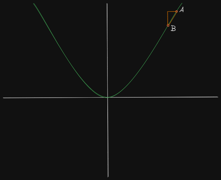
But now we try something new, Gradient Descent. We will find the gradient w.r.t to the positions at A and B, and intuitively we can see that B can be reached by :
This procedure of repeatedly evaluating the gradient and then updating the parameters essentially is nothing but Gradient Descent!
How much we step and how far we want to go, is decided by \(\alpha\), which is coined as learning rate. Larger the value, more step-size we take, indication a further down B.
Code
We first get the predictions on the whole training data, then we calculate the loss using some loss function. Finally, we update the weights in the direction of the gradients to minimize the loss. We do this repeatedly for some predefined number of epochs.
for epoch in range(no_of_epochs):
	prediction=model(training_data)
	loss=L(prediction,truth_values)
	W_grad=evaluate_gradient(loss)
	weights-=learning_rate*W_grad
What’s the problem with this method?
What if we have millions of data? We can see that the loss function will be counted over the whole dataset, just for one parameter update. This will be computationally difficult and to address this challenge we come up with a new method.
Approach 5 - Stochastic Gradient Descent
Logic
In Stochastic Gradient Descent(SGD), we divide our training data into sets of batches.
SGD has two main components :
- We have to divide the training data into batches
- For each batch of data,
i) Find out the predictions on the data and find out the loss
ii) Calculate the gradients, based on the loss
iii) Take a step in the opposite direction of gradients to minimize loss
Code (Simple)
for epoch in range(no_of_epochs):
	for input_data,labels in training_dataloader: #dataloader divides everything into batches
		prediction=model(training_data)
		loss=L(prediction,truth_values)
		W_grad=evaluate_gradient(loss)
		weights-=learning_rate*W_grad
Code (Pytorch)
In Pytorch, you can simply use the torch.optim.Optimizer class for all your optimizer needs. It has the necessary step and zero_grad functions needed for your code
#Pytorch Implementation
model = create_model()
optimizer = torch.optim.SGD(model.parameters(), lr=1e-4)

for input_data, labels in train_dataloader:
    preds = model(input_data)
    loss  = L(preds, labels) #finding out loss
    loss.backward() #gradient
    optimizer.step() #updates the weights by taking step
    optimizer.zero_grad() #resets the grad values to 0 for each epoch
Problems with SGD
Problem 1
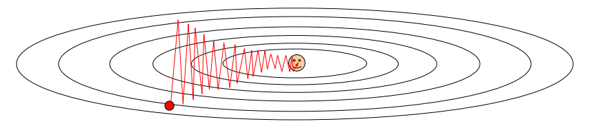
What if loss changes quickly in one direction and slowly in another? What does gradient descent do?
Ans : The loss function will move slowly along the shallow direction (where the gradient value is small), and it will start jittering. You will be able to notice a zig zag behaviour, as the gradients will be large in that direction and we waste a lot of training time hence.
Problem 2
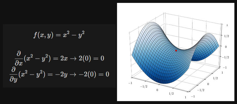
What if the loss function has a local minima or saddle point?
Ans : Since that point has zero gradient, the gradient descent will stop and the optimizer gets stuck, in the case of local minima.
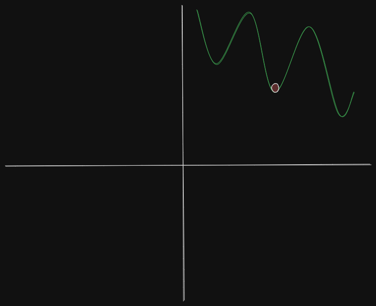
In the case of a saddle point too, we can see it has 0 gradient too, so it will definitely get stuck there.
Problem 3
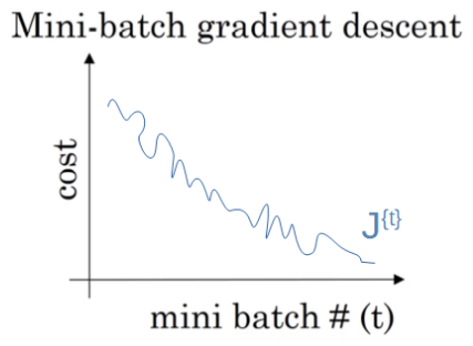
The gradients are calculated from small batches so it has been noticed that they will have a considerable amount of noise in them as well