All about Quantization

a guide into how quantization occurs in llms

shortening memory aka parameters

10 min read

Oct 9, 2024

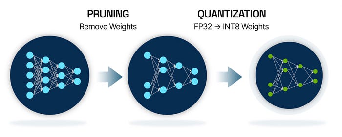
Why do we need it?

It is now the age of LLMs, anywhere you work, you will be using LLMs in some way or the other. Models nowadays have several billions of parameters, which can be challenging for anyone to store, additionally, we also need to store the activations after the input and weights equally large as the weights.

Our goal is to represent billions of numbers, by minimising the space taken by a given value. For that, we must start by understanding how values are stored in the first place.

Types of Numerical Values

Each value is nothing but a floating-point number (or, decimal). These values are represented by binary digits called, bits. Each of the bits can represent either of 3 different types of values — sign, exponent or mantissa

INT8

Press enter or click to view image in full size

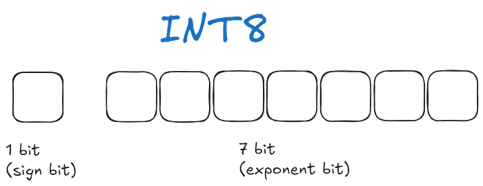
The sign bit represents the sign of the number, we can find the sign by taking it to the power of -1. The sign bit of 0 means (-1)⁰ = 1 ~ positive number, and the sign bit of 1 will mean negative numbers.

It has no mantissa, only the integral part of exponent bits.

FP16 (Float 16bit)

Press enter or click to view image in full size

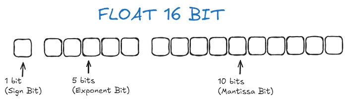
The sign bit is the same as INT8.

The exponent bit refers to the integral part of the number and can be found easily by converting binary to decimal.

The mantissa bit refers to the fractional part of the number and can be found easily by converting binary to decimal.

FP32 (Float 32bit)

Press enter or click to view image in full size

It’s the same as FP16, but it has space for more digits and hence has more precision as compared to FP16. Precision is the distance between two neighbouring values, if the distance is very low, it means high precision and vice versa.

The more bits we have available, the more the range of values we can represent.

We can find out how much memory a n-bit system system will need according to the formula below!

This means an FP32 model with 70 billion parameters will take around 280GB of space. That means we need to use a lower-bit system, but we know as we go lower, we start losing accuracy/precision. That is where quantization comes in. That’s what we aim to do.

Then let’s try to minimise our bits from FP32 to its lower bit types!

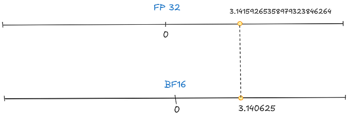
BF16

This is a special type of FP16, called truncated FP32. Its speciality is that it has the same range as FP32 but at half the precision.

Press enter or click to view image in full size

FP16

Press enter or click to view image in full size

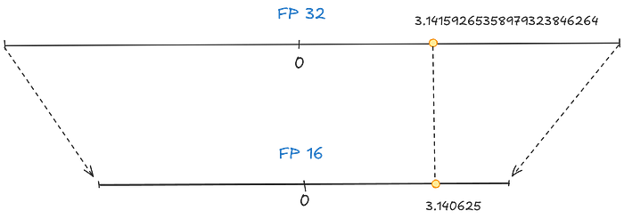
This is called half-precision, as we go from FP32 to FP16. We can notice the value taken by FP16 is much less than that of FP32.

INT8

Press enter or click to view image in full size

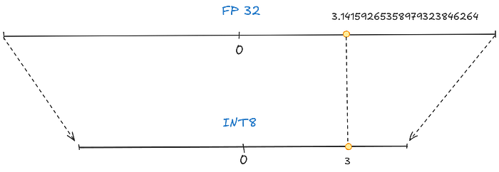
This is our last step of reduction, we are in integers ~ 32 bits to 8 bits. We noticed that we squeezed the large value of FP32 into smaller and smaller bits. To find the corresponding value of the FP32 number in lower bits, we need to find a linear mapping from FP32 to INT8.

Mapping Methods

Symmetric Quantization

In symmetric quantization, the mapping is done in such a way that the ranges are centred, i.e. 0 of FP32 is equal to 0 of INT8. We will be doing a specific type of symmetric quantization, called absmax quantization.

Press enter or click to view image in full size

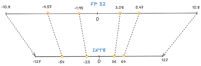
In a list of numbers [-4.57,3.08,5.47,-1.95,10.8], we find the highest absolute value (α) as the range of FP32 to perform the mapping.

First, we need to find a scale factor(s), which the formula can find:

where b is the number of bytes to which we want to quantize, and α is the highest absolute value. The formula is obvious, as we are dividing the total bits by the highest value to show how much 1-bit amounts to scale in the lower scale.

The final quantized value then comes out to be

To dequantize, we can just divide by the scaling factor of s

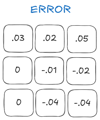
Let’s see a batch of quantization and dequantization

Press enter or click to view image in full size

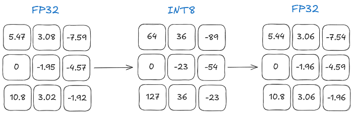
We can see that the values 3.02 and 3.08 both get assigned to 36 and lose their original values due to a lessening of precision. This is called quantization error, which is the difference between the original and dequantized values. The lower the number of bits, the more quantization error we have.

Asymmetric Quantization

In asymmetric quantization, we don’t center around 0, instead the mapping is done between the minimum(β) and maximum(α) values from FP32 to the maximum and minimum of the quantized values.

Press enter or click to view image in full size

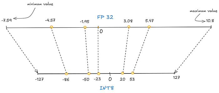
You can notice the 0 in FP32 is no more than 0 in INT8. The minimum and maximum values have different distances from 0 in INT8 and hence it becomes asymmetric.

The new and adjusted scale factor(s) becomes :

The formula for the zero-point comes out to be :

The final quantized value becomes :

To dequantize the values from INT8 back to FP32, we will be using the below formula :

Range Mapping and Clipping

We saw how an entire range of values in a vector can easily be mapped to a lower-bit system, but now we have a problem with that system too. The problem is Outliers.

Let’s say you have a set of values :

[-4.57,-.195,3.08,5.47,55.48,256] You can see how 256 is much larger than the rest of the values, leading to most of the other values getting mapped to the same number(0 in our case), in any quantization method, and they will lose their only differentiating factor!

We clip values so all the outliers get the same value to avoid this. If we set the range to be [-6,6] in the earlier case, all the values more than 6 and less than -6 will automatically get assigned 127 or -127 respectively, regardless of what value they carry.

Press enter or click to view image in full size

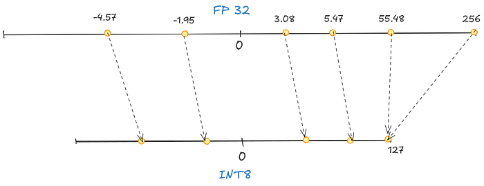
Hence we reduce the quantization error of non-outliers by a huge margin, but the error of outliers increases by a lot too.

Calibration

In the last example, I randomly chose a range of [-6,6] but that is now how it happens. The process of selecting the range is called Calibration which finds the range, that will have the least quantization error.

Techniques (Weights and Biases)

In an LLM, most of the data that is stored is just the weights and biases(as they are static values). There will be significantly less number of biases rather than there are weights, hence biases will be kept in INT16 or higher. So our target of quantization is nothing but the weights.

Get neuralnetworks’s stories in your inbox

Join Medium for free to get updates from this writer.

Remember me for faster sign in

Some Techniques to do it are : 1. First choose a percentile of the input range.

Then optimize the MSE between the original and quantized weights
Minimize the KL Divergence between the original and quantized weights.

Dealing with Activations

Unlike static weights, activations will vary with each set of input entered into the model, making them hard to quantize. Since they are updated every time, we only know their value after the input data has already been passed

Now we will try to calibrate the quantization of weights and activations, using two new methods!

Post-Training Quantization (PTQ)

It quantized the model’s params after the training of the model had been done. Quantization of the weights is done either by symmetric or asymmetric quantization. Quantization of the activations can be done by two different methods here :

Static Quantization
Dynamic Quantization

Static Quantization

Static Quantization never calculates the zero-point nor the scale factor during the inference, but does it beforehand. To find such values, a predetermined dataset is used and the model collects potential distributions from them. After these values are obtained, we find out the optimum zero-point and scale factor values to perform our quantization. Hence, the scale factor and zero-point values are never recalculated but are used globally over all the activations present so that they can be quantized.

Press enter or click to view image in full size

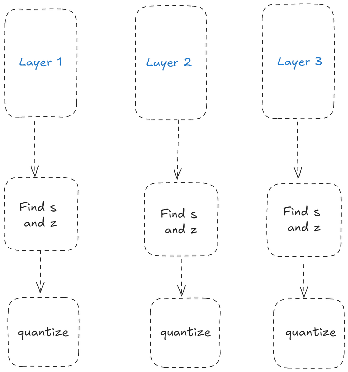
Dynamic Quantization

After the input data passes any hidden layer, all its activations are stored. The values collected are then used to calculate the zero-point and scale factor values that are needed to quantize the output value. The process is repeated every time the input data passes a ew layer. Hence, in this case, each layer will have it’s own zero-point and scale factor values.

Press enter or click to view image in full size

Quantization Aware Training (QAT)

One major problem in the last approach of PTQ was that the model doesn’t care about what and how the training actually happens, hence comes Quantization Aware Training. Here, it tries to quantize the values during the training procedure, instead of after the training procedure in PTQ. This is more kinda more accurate than PTQ as quantization is considered during the training phase itself.

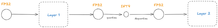
How does it work?

During the traing procedure, we add some quantization between the layers, called Fake Quants. It quantizes the weights from FP32 to lower bit representation and then back to FP32. This process actually leads to the quantization process being done during training. This leads to far lesser quantization errors than in PTQ, in lower precisions, like INT 4.

Press enter or click to view image in full size

Specific Quantization Methods

GGUF

GGUF offloads any layer from your LLM to your CPU, hence making your system compatible to run LLms even with low VRAM. Both CPU and GPU is used during this method

How does it work?

Press enter or click to view image in full size

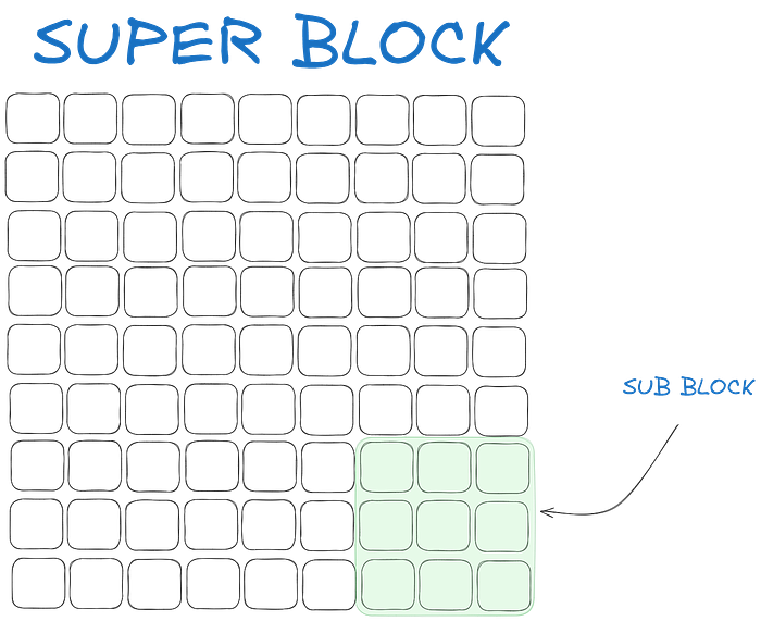
The total weights are broken into blocks, each called Super Blocks.They are further broken down into blocks, called Sub Blocks. From each of these sub blocks, we find their scale factor and maximum absolute value. Now to quantize a subblock, we use the absmax quantization like before. But the twist is the scale factor of each sub-block for quantization is not used in the quantization of the sub-block, instead, we use the scale factor of the superblock!

GPTQ

This is mainly used to convert higher precisions to 4-bit systems. It utilizes asymmetric quantization and does it in such a manner so that each layer is quantized before it moves to the next layer.

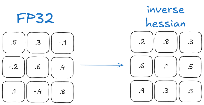
The layer weights are first converted into inverse-Hessian form [2nd order derivative and shows the importance of each weight in the layer]. Weights with small values have more importance as small changes result to large ones in model performance.

Press enter or click to view image in full size

We will move row-wise, so let’s look at the first row. We will quantize the first element and then dequantize it. After this, we calculate the quantization error(q) which will be normalized by its weight in the inverse hessian (h_1).

Now we redistribute the quantization error over all the other weights in the row.

We will keep reiterating this process until all the values have been quantized. The main thing that makes GPTQ good is that even if one weight has some quantization error, the weights related to that weight are immediately updated!